
Full Text View
Volume 28 Issue 3-4 (March/April 2018)
GSA Today
![]()
Article, pp. 4-10 | Abstract | PDF (4.8MB)
Cosmogenic nuclides indicate that boulder fields are dynamic, ancient, multigenerational features
Cover Image
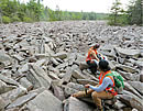
Table of Contents
- Introduction
- Geologic and Physiographic Setting
- Application of Cosmogenic Nuclides to Boulder Fields
- Methods
- Results
- Discussion
- Acknowledgments
- References Cited
Search GoogleScholar for
Search GSA Today
Abstract
Boulder fields are found throughout the world; yet, the history of these features, as well as the processes that form them, remain poorly understood. In high and mid-latitudes, boulder fields are thought to form and be active during glacial periods; however, few quantitative data support this assertion. Here, we use in situ cosmogenic 10Be and 26Al to quantify the near-surface history of 52 samples in and around the largest boulder field in North America, Hickory Run, in central Pennsylvania, USA.
Boulder surface 10Be concentrations (n = 43) increase downslope, indicate minimum near-surface histories of 70–600 k.y., and are not correlated with lithology or boulder size. Measurements of samples from the top and bottom of one boulder and three underlying clasts as well as 26Al/10Be ratios (n = 25) suggest that at least some boulders have complex exposure histories caused by flipping and/or cover by other rocks, soil, or ice. Cosmogenic nuclide data demonstrate that Hickory Run, and likely other boulder fields, are dynamic features that persist through multiple glacial-interglacial cycles because of boulder resistance to weathering and erosion. Long and complex boulder histories suggest that climatic interpretations based on the presence of these rocky landforms are likely oversimplifications.
* Now at Pinnacle Potash International, Ltd., 111 Congress Ave, Suite 2020, Austin, Texas 78701, USA
Manuscript received 31 Mar. 2017. Revised manuscript received 21 Aug. 2017. Manuscript accepted 4 Oct. 2017. Posted online 20 Dec. 2017
© The Geological Society of America, 2017. CC-BY-NC.
Introduction
Areas outside the maximum extent of Pleistocene glaciation contain landforms thought to have been produced during cold climate periods (Clark and Ciolkosz, 1988) by frost action and mass wasting (periglaciation). These features, particularly unvegetated boulder fields, boulder streams, and talus slopes (areas of broken rock distinguished by differences in morphology and gradient [Wilson et al., 2016]), are believed to be largely inactive today (Braun, 1989; Clark and Ciolkosz, 1988).
Boulder fields have been documented throughout the world, including Australia (Barrows et al., 2004), Norway (Wilson et al., 2016), South Africa (Boelhouwers et al., 2002), the Falkland Islands (Wilson et al., 2008), Italy (Firpo et al., 2006), Sweden (Goodfellow et al., 2014), and South Korea (Seong and Kim, 2003). Hundreds of such fields exist in eastern North America (Nelson et al., 2007; Potter and Moss, 1968; Psilovikos and Van Houten, 1982; Smith, 1953); however, both the time scale and mechanism of boulder field formation remain poorly understood because few quantitative data constrain the age of boulder field formation or evolution.
Boulder field formation is usually explained by one of two process models, both of which invoke periglaciation as a catalyst for boulder generation and transport (Rea, 2013; Wilson, 2013): (1) boulders fall from a bedrock outcrop upslope of the field and are transported downslope by ice-catalyzed heaving and sliding (Smith, 1953); or (2) boulders form as corestones underground, are unearthed by the progressive removal of surrounding saprolite, and are later reworked (André et al., 2008). However they form, boulder fields are likely altered over time by in situ rock weathering, erosion, accumulation of unconsolidated soil/regolith, and perhaps by periglacial action or glaciation during cold periods (André et al., 2008).
Here, we report 52 measurements of 10Be and 25 measurements of 26Al in boulders and outcrops in and near the Hickory Run boulder field. Data show that boulders in the field have moved over time and can have cosmogenic nuclide concentrations equivalent to at least 600 k.y. of near-surface history. We conclude that boulder fields survive multiple glacial-interglacial cycles, calling into question their utility as climatic indicators.
Geologic and Physiographic Setting
Hickory Run boulder field is ~2 km south of the Last Glacial Maximum (LGM) Laurentide Ice Sheet boundary (Pazzaglia et al., 2006; Sevon and Braun, 2000) in east-central Pennsylvania, USA (Fig. 1A), a temperate, forested, inland region of the Atlantic passive margin. The field sits on a low-relief upland surface underlain by gently folded, resistant Paleozoic sandstones and conglomerates.
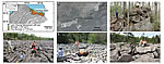 Figure 1
Study site. (A) Hickory Run location in relation to the extent of the Last Glacial Maximum (LGM) (26 ka, Corbett et al., 2017b), Illinoian (130 ka?), and pre-Illinoian glaciations, after Sevon and Braun (2000). Hickory Run is 2 km south of the LGM boundary and is mapped within the Illinoian and pre-Illinoian glaciations. (B) Locations of photographs; (C) tors on a ridgeline 700 m NE of the field; (D) elongate, angular, large boulders upslope; (E) small, rounded boulders downslope; and (F) massive, angular conglomeritic boulders in the SE sub-field.
The field is an elongate, 550- by 150-m-wide, nearly flat (1°) expanse of boulders in the axis of a small valley (Fig. 1) with ~30 m of relief (Smith, 1953). Boulders in the field range from <1 to >10 m long and are hard, gray-red, medium-grained sandstone and conglomeratic sandstone from the Catskill formation (Sevon, 1975), as are the adjacent ridgelines. Upslope boulders at the northeast end of the field (Fig. 1D) are generally more angular than those downslope to the southwest (Fig. 1E) (Wedo, 2013), which are mostly subrounded and underlain by small, polished clasts with a red weathering rind (Fig. 1E). There is a distinct subsection of the field to the southeast with boulders mostly >5 m long; these appear to be bedrock shattered along bedding planes (Fig. 1F). The field is surrounded by coniferous forest with stony loam soils (NRCS, 2014).
Glacial erratics are found south of Hickory Run (Pazzaglia et al., 2006; Sevon and Braun, 2000), indicating that it was covered by ice at least once, although the timing of ice advances is not well known (Braun, 2004), and we found no obvious erratics in the field. The last glaciation to override Hickory Run is mapped as Illinoian (ca. 150 ka; Fig. 1A), though it is possible that it was 400 ka (Braun, 2004). South of the boulder field, reversed magnetic polarity deposits indicate that the oldest, most extensive glaciation was in the early Pleistocene (likely >900 ka); there is another event mapped between the Illinoian event and the >900 ka event, distinguished by proglacial lake sediments of normal polarity, likely <740 ka (Braun, 2004).
Application of Cosmogenic Nuclides to Boulder Fields
Cosmogenic nuclides are produced predominately in the uppermost meters of Earth’s surface by cosmic ray bombardment (Gosse and Phillips, 2001; Lal and Peters, 1967). Nuclides build up over time and can be used to provide age control for surficial deposits; however, such dating requires that at the time of initial surface exposure, rock contained few if any nuclides (Lal, 1991). This is not the case for boulder fields because both models of development (see Introduction) include initial cosmic-ray exposure before incorporation of blocks into the field (on cliffs or below a weathered regolith mantle).
The pertinent question becomes, “Where were the sampled boulders when they received the cosmic ray dosing that accounts for the 10Be and 26Al concentrations they contain today?” This question arises because there is no unique and agreed upon process model for boulder field development. If boulders were sourced from outcrops upslope of the field and moved downfield, they inherited nuclides from exposure on the outcrops. If boulders originated in place, they inherited nuclides from subsurface exposure. In either case, measured nuclide concentrations do not allow direct dating of the time any boulder became exposed as part of the boulder field; rather, they allow for the calculation of minimum total near-surface histories for each sampled boulder. Such histories integrate cosmic-ray exposure and express it as the equivalent of uninterrupted surface exposure. These times are minima because we know boulders eroded and also experienced less than surface production rates before they were exhumed, when they were covered by other boulders, and/or when they flipped during transport.
If rock surfaces experience burial before, during, or after exposure, by flipping or cover with soil, snow, ice, or other boulders, such complex histories can be detected by measuring two isotopes with different half-lives in the same sample (Bierman et al., 1999; Nishiizumi et al., 1991). Such analyses most commonly employ 26Al and 10Be, which are produced in quartz at a ratio of ~7:1 (Argento et al., 2013; Corbett et al., 2017a). Because the 26Al half-life, 0.71 m.y. (Nishiizumi et al., 1991), is about half that of 10Be, 1.38 m.y. (Chmeleff et al., 2009; Korschinek et al., 2010), if an exposed sample is buried, the 26Al/10Be ratio will decrease; if that sample is re-exposed, production of nuclides begins again and the ratio increases. Because of the relatively long half-lives of 26Al and 10Be, the 26Al/10Be ratio is only sensitive to burial by meters of material for >100 k.y. (Lal, 1991).
Published measurements of cosmogenic nuclides, made on samples collected from rock surfaces in high-latitude boulder fields, suggest that some blocks were exposed to cosmic rays relatively recently, while others have concentrations consistent with near-surface histories extending over hundreds of thousands of years. For example, 36Cl concentrations in 18 Australian boulder stream samples reveal a cluster of minimum limiting exposure histories around 21 ± 0.5 ka (LGM), while other samples from the same field have minimum total near-surface histories of 60–480 ka (Barrows et al., 2004). Samples from boulder streams in the Falkland Islands (n = 16) have 10Be histories of 42–730 ka (Wilson et al., 2008). A Korean boulder field has 10Be histories (n = 4) between 38 and 65 ka (Seong and Kim, 2003), while samples from Swedish boulder fields have histories of 33 and 73 ka (n = 2) (Goodfellow et al., 2014). Analysis (n = 15) of paired 26Al and 10Be in block streams suggests some boulders have histories that include either exposure under cover and/or burial after near-surface exposure (Goodfellow et al., 2014; Seong and Kim, 2003; Wilson et al., 2008).
Methods
We sampled in and around the Hickory Run boulder field in eight slope-normal transects, collecting a total of 52 samples by removing the surficial few centimeters of rock. Of these samples, 30 were from boulders in the main field, six were from the southeastern sub-field, seven were from boulders in the surrounding forest, five were from bedrock tors cropping out on a ridgeline 700 m NE (Fig. 1C), and one was from the bottom of a boulder accompanied by three underlying clasts (Fig. 2A). We photographed and recorded the dimensions, sub-meter resolution UTM coordinates, sample thickness, and lithology of each boulder. Additionally, we used eCognition software to automatically extract boulder outlines from aerial imagery to test for trends in boulder size and orientation.
 Figure 2
Measurement of boulder HR10 and underlying clasts. (A) Photograph of boulder HR10 on top of clasts; (B) side view of HR10 samples and underlying clasts; (C) 10Be production decreases exponentially with depth. The black dashed line represents the 10Be concentrations expected in HR10B and samples 10C1–C3 if they remained in place at depth for their entire histories. (D) Depth profile assuming the boulder flipped 180 ° at 25 ka—the concentration in HR10T is too high to have flipped then. (E) Sample HR10T aligns with the depth profile assuming the boulder flipped at 200 ka.
We purified quartz (Kohl and Nishiizumi, 1992) and extracted 10Be and 26Al (Corbett et al., 2016) at The University of Vermont. We measured 10Be/9Be ratios at Lawrence Livermore National Laboratory, normalizing them relative to ICN standard 07KNSTD3110 with an assumed value of 2.85 × 10⁻¹² (Nishiizumi et al., 2007). We corrected our data using process blanks (see GSA Data Repository1 Table DR1) and processed four replicates to test reproducibility; the difference between replicates ranged from <1%–4% (mean 2%). We then selected the boulder bottom and clast samples (n = 4) along with a subset of upslope (n = 10) and downslope (n = 11) boulder samples for 26Al/27Al analysis at PRIME Lab. Minimum near-surface histories were calculated using the CRONUS Earth online calculator (http://hess.ess.washington.edu/), wrapper script 2.2, main calculator 2.1, constants 2.2.1 (see Balco et al. [2008]) based on the constant production rate model (Lal, 1991; Stone, 2000) using the regional northeastern U.S. production rate (Balco et al., 2009).
--------
1 GSA Data Repository Item 2017393, a detailed description of methodology, is online at www.geosociety.org//datarepository/2017/.
Results
Boulders at Hickory Run have experienced widely varying and substantial near-surface exposure. Hickory Run samples have 10Be concentrations ranging from 0.44 to 3.26 × 10⁶ atoms g−1 (Fig. 3), the equivalent of between 70 and 600 k.y. of surface exposure.
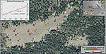 Figure 3
10Be concentration (105 atoms g−1) of Hickory Run boulders and tors; red dots indicate higher 10Be concentration; green dots indicate lower. Insets show location of tors (Fig. 1C) relative to the main boulder field and positive correlation between 10Be concentration and downslope distance.
There is no significant correlation between 10Be concentration and boulder lithology, size, or proximity to the edge of the field. Boulders downslope are more rounded, smaller (Fig. DR1 [see footnote 1]), and have more developed weathering rinds than those upslope, suggesting that boulder weathering increases downslope. We also observe spatial trends in boulder orientation; downslope boulders align with the main axis of the field (NE-SW), whereas upslope boulders align E-W
(Fig. DR1 [see footnote 1]).
Our 10Be results support the inference of increased weathering and near-surface exposure time downfield. The strongest correlation we observe is between downfield distance and 10Be concentration (r2 = 0.45; Fig. 3); additionally, 10Be concentrations within the main body of the field become increasingly different with distance between boulders (Fig. DR2 [see footnote 1]). Boulders upfield (n = 10) include the two lowest measured 10Be concentrations (0.4 ± 0.07 × 10⁶ atoms g−1; Fig. 4) whereas downfield boulders contain much more 10Be, averaging 2.1 ± 0.6 × 10⁶ atoms g−1. Concentrations on ridgeline tors and in the southeastern sub-field tend to be lower than the main body of the field (Fig. 4).
 Figure 4
Summed probability plot of 10Be concentrations (A) in tors, (B) of the three furthest upslope boulder transects, and (C) of the two furthest downslope. Red curves represent single 10Be measurements with 2σ internal error; the black line represents the sum of all samples.
Our measurements of boulder HR10 and of the clasts below it are inconsistent with simple exposure in place (Fig. 2) and imply movement and flipping of the boulder. The measured 10Be concentration in sample HR10B (from the underside of the boulder, 0.39 m below the surface) is 170% of what it would be if the boulder had received all of its exposure as currently oriented (Table DR1 [see footnote 1]). Clasts C1, C2, and C3 have more than triple the expected 10Be concentration than if they had been continuously irradiated underneath the boulder; all three have higher concentrations than the sample from the top of the boulder. The boulder and clasts could not have been exposed and irradiated only in their current position.
Concentrations of 26Al range from 3.00 to 19.3 × 10⁶ atoms g−1 (n = 25), and correlate well with 10Be measurements (r2 = 0.99). 26Al/10Be ratios range from 5.4 to 7.3. When plotted on a two-isotope diagram (Fig. 5), all but five samples fall below the upper constant exposure line, consistent either with exposure followed by erosion (between the upper and lower lines), with at least one episode of burial after initial exposure, or with exposure under cover followed by exhumation. Samples from the top of the field (n = 10) have an average 26Al/10Be of 6.61 ± 0.46, whereas those from the bottom of the field (n = 11) have an average 26Al/10Be of 5.96 ± 0.31 (separable at 95% confidence, Student’s t-test). In part, this decrease reflects longer near-surface histories of boulders downfield.
 Figure 5
Measured 26Al/10Be plotted against measured 10Be concentrations (n = 25). Plot is based on a local production rate of six atoms g−1 y−1 and surface production ratio of 7.0 (Argento et al., 2013). The thick black line indicates constant surface exposure, and the line beneath it marks the end of the “steady erosion envelope”; points beneath this envelope have had at least one period of burial or shielding during or after exposure. Thin lines represent the trajectory that a sample would follow if buried, and dotted lines indicate burial isochrons of 0.5, 1.0, and 1.5 m.y. assuming surface exposure followed by deep burial (top to bottom).
Discussion
Cosmogenic nuclide measurements, when considered along with field observations, provide a means to infer how boulder fields change over time. For example, boulders at Hickory Run are more rounded, smaller, and thus more weathered downfield than upfield; the downfield increase in 10Be concentration suggests the importance of near-surface residence time in physical and chemical boulder weathering. The decrease in 26Al/10Be ratios downfield indicates that boulders there have experienced more complex exposure histories, including erosion, exhumation, burial, and/or flipping, than upfield boulders. Changes in boulder long-axis alignment downfield likely indicate at least some downfield, and thus downslope, boulder transport.
Multiple cosmogenic measurements on a single boulder (HR10) reveal more about boulder history and boulder field processes. Measurements of samples from the top and bottom of the boulder, as well as the underlying clasts, demonstrate that it has changed position and not simply weathered in place. Although there is no unique solution, this disparity in concentration between the top and bottom of the boulder can be resolved if, ~200,000 years ago, it flipped after initial exposure and was then deposited on top of the clasts now underlying it (Fig. 2 and Tables DR3–DR5 [see footnote 1]). High nuclide concentrations in clasts under the boulder provide further evidence for boulder movement. Nuclide concentrations in clasts HR10 C1, C2, and C3 are comparable to those of nearby surface boulders, and their 26Al/10Be ratios are indistinguishable from the production ratio. This is likely because the clasts spent most of their history near the surface and still receive substantial cosmic ray dosing through the overlying 48 cm of rock.
The positive linear relationship between 10Be concentration and distance downfield allows calculations of the rate at which the field changes over time. Assuming boulders were sourced from outcrops upslope of the field, the relationship between 10Be concentration and distance downslope can be interpreted as a rate of transport (Jungers et al., 2009; Nichols et al., 2005; West et al., 2013). Given a local 10Be production rate of 6 atoms g−1 y−1 and a regression slope of 4050 atoms m−1 (Fig. 3), the average rate of boulder movement is ~15 mm y−1 presuming the boulders remain exposed at the surface, and slower if the boulders were buried or flipped during transport as suggested by 26Al/10Be ratios, discussed above. Alternatively, if the field is the result of progressive up-field stripping of regolith and the boulders have remained in place, then the speed represents the rate at which the bedrock/regolith boundary moved upslope.
At Hickory Run, minimum total near-surface histories are varied and long. They range from 70 to 600 k.y. with a mode between 120 and 210 ka. Such histories are similar to those reported in boulder field samples collected elsewhere (Wilson et al., 2008) (Fig. 6) and together suggest that boulder fields are persistent features that can survive multiple glacial cycles. Boulders at Hickory Run have much longer minimum total near-surface histories than sandstone outcrops in the central Appalachian Mountains, but have minimum total near-surface histories only slightly greater than quartzite outcrops in the region (Portenga et al., 2013), consistent with the indurated nature of rock exposed at Hickory Run (Fig. 6). The similarity of near-surface residence time (Fig. 6) between quartzite outcrops and Hickory Run boulders suggests a different approach to interpreting boulder fields—considering them as fractured outcrops, unmantled by soil and regolith. In this framework, boulder field longevity is controlled by the resistance of boulders to erosion over time.
 Figure 6
Summed probability plots of minimum total near-surface history derived from 10Be. Red curves represent single 10Be measurements with 2σ internal error; the black line represents the sum of all samples. (A) All Hickory Run samples. (B) Quartzite bedrock outcrops. (C) Sandstone outcrops. (D) Other boulder field samples (Barrows et al., 2004; Goodfellow et al., 2014; Seong and Kim, 2003; Wilson et al., 2008). (E) Stable δ18O ratios in deep sea foraminifera (Railsback et al., 2015). Even numbers represent cold glacial stages; odd numbers are interglacials. LGM—Last Glacial Maximum.
Although most prior research suggests that boulder fields result from periglacial activity (Braun, 1989; Clark and Ciolkosz, 1988), extant cosmogenic data are largely agnostic as to the timing of boulder generation. The absence of LGM histories among the 52 Hickory Run samples we analyzed could indicate a lack of new boulder generation during the most recent cold period. Conversely, the absence of LGM histories may reflect pre-exposure of boulders, at depth if they are unroofed, or upslope if they moved downslope from source outcrops. Comparison of the cumulative probability distribution of all boulder analyses (Fig. 6) to the marine oxygen
isotope record of climate shows no obvious correlation of boulder histories with climate except that the mode of boulder histories at Hickory Run is generally consistent with the Illinoian cold period (130–190 ka, MIS 6). Either the complexity of boulder histories (flipping, erosion, exhumation) blur any coherent time signal in the data or perhaps boulder field generation is not strictly a periglacial phenomenon.
Hickory Run is mapped within the Illinoian glacial margin (Sevon and Braun, 2000) and, if mapping and dating of the Illinoian are correct, would have been under glacial ice ca. 150 ka (Fig. 1A). The absence of erratics within the field and the presence of boulders with minimum histories far exceeding 150 k.y. suggest that the “Illinoian” in this part of Pennsylvania is likely older than previously assumed, a possibility given the lack of quantitative age constraints on old glaciations (Sevon and Braun, 2000). Alternately, if the mapping were correct, then any overriding Illinoian ice must have been cold-based and non-erosive, as the boulder field was preserved rather than eroded. The preservation of block streams under cold-based ice is possible (Kleman and Borgström, 1990), and portions of the southern Laurentide ice sheet were likely cold-based (Colgan et al., 2002; Bierman et al., 1999, 2015).
High concentrations of cosmogenic nuclides in samples collected from Hickory Run highlight the stability and persistence of this landform, which has survived at least one, and likely several, glacial/interglacial cycles. Cosmogenic nuclide measurements provide limited information about the timing of boulder field activity (insufficient to confirm it is a periglacial feature), but clearly indicate that Hickory Run and at least some other boulder fields throughout the world are ancient, dynamic, multigenerational features, the longevity of which appears to be controlled by the resistance of their boulders to erosion.
Acknowledgments
We thank N. West and M. Bruno for field assistance. We also thank our anonymous reviewers, who greatly improved the quality of this manuscript, as well as Noel Potter for his input on this mysterious feature! This research was supported by NSF-EAR1331726 (S. Brantley) for the Susquehanna Shale Hills Critical Zone Observatory. M.W. Caffee was supported by NSF-EAR1560658.
References Cited
- André, M.-F., Hall, K., Bertran, P., and Arocena, J., 2008, Stone runs in the Falkland Islands: Periglacial or tropical?: Geomorphology, v. 95, no. 3–4, p. 524–543, https://doi.org/10.1016/j.geomorph.2007.07.006.
- Argento, D.C., Reedy, R.C., and Stone, J.O., 2013, Modeling the Earth’s cosmic radiation: Nuclear Instruments & Methods in Physics Research, Section B, Beam Interactions with Materials and Atoms, v. 294, p. 464–469, https://doi.org/10.1016/j.nimb.2012.05.022.
- Balco, G., and Rovey, C.W., 2008, An isochron method for cosmogenic nuclide dating of buried soils and sediments: American Journal of Science, v. 308, p. 1083–1114, https://doi.org/10.2475/10.2008.02.
- Balco, G., Stone, J.O., Lifton, N.A., and Dunai, T.J., 2008, A complete and easily accessible means of calculating surface exposure ages or erosion rates from 10Be and 26Al measurements: Quaternary Geochronology, v. 3, p. 174–195, https://doi.org/10.1016/j.quageo.2007.12.001.
- Balco, G., Briner, J., Finkel, R.C., Rayburn, J.A., Ridge, J.C., and Schaefer, J.M., 2009, Regional beryllium-10 production rate calibration for late-glacial northeastern North America: Quaternary Geochronology, v. 4, p. 93–107, https://doi.org/10.1016/j.quageo.2008.09.001.
- Barrows, T.T., Stone, J.O., and Fifield, L.K., 2004, Exposure ages for Pleistocene periglacial deposits in Australia: Quaternary Science Reviews, v. 23, no. 5–6, p. 697–708, https://doi.org/10.1016/j.quascirev.2003.10.011.
- Bierman, P.R., Marsella, K.A., Patterson, C., Davis, P.T., and Caffee, M., 1999, Mid-Pleistocene cosmogenic minimum-age limits for pre-Wisconsinan glacial surfaces in southwestern Minnesota and southern Baffin Island; a multiple nuclide approach: Geomorphology, v. 27, no. 1–2, p. 25–39, https://doi.org/10.1016/S0169-555X(98)00088-9.
- Bierman, P.R., Davis, P.T., Corbett, L.B., Lifton, N.A., and Finkel, R.C., 2015, Cold-based Laurentide ice covered New England’s highest summits during the Last Glacial Maximum: Geology, v. 43, no. 12, p. 1059–1062, https://doi.org/10.130/G37225.1.
- Boelhouwers, J., Holness, S., Meiklejohn, I., and Sumner, P., 2002, Observations on a blockstream in the vicinity of Sani Pass, Lesotho Highlands, southern Africa: Permafrost and Periglacial Processes, v. 13, no. 4, p. 251–257, https://doi.org/10.1002/ppp.428.
- Braun, D.D., 1989, Glacial and Periglacial Erosion of the Appalachians: Geomorphology, v. 2, p. 233–256, https://doi.org/10.1016/0169-555X
- (89)90014-7.
- Braun, D.D., 2004, The glaciation of Pennsylvania, USA: Developments in Quaternary Sciences, v. 2, p. 237–242, https://doi.org/10.1016/S1571-0866(04)80201-X.
- Chmeleff, J., von Blanckenburg, F., Kossert, K., and Jakob, D., 2009, Determination of the 10Be half-life by multicollector ICP-MS and liquid scintillation counting: Nuclear Instruments & Methods in Physics Research, Section B, Beam Interactions with Materials and Atoms, v. 268, no. 2, p. 192–199, https://doi.org/10.1016/j.nimb.2009.09.012.
- Clark, G.M., and Ciolkosz, E.J., 1988, Periglacial geomorphology of the Appalachian Highlands and Interior Highlands south of the glacial
- border—A review: Geomorphology, v. 1, no. 3, p. 191–220, https://doi.org/10.1016/0169-555X(88)90014-1.
- Colgan, P.M., Bierman, P.R., Mickelson, D.M., and Caffee, M., 2002, Variation in glacial erosion near the southern margin of the Laurentide Ice Sheet, south-central Wisconsin, USA: Implications for cosmogenic dating of glacial terrains: Geological Society of America Bulletin, v. 114, no. 12, p. 1581–1591, https://doi.org/10.1130/0016-7606(2002)114<1581:VIGENT>2.0.CO;2.
- Corbett, L.B., Bierman, P.R., and Rood, D.H., 2016, An approach for optimizing in situ cosmogenic 10Be sample preparation: Quaternary Geochronology, v. 33, p. 24–34, https://doi.org/10.1016/j.quageo.2016.02.001.
- Corbett, L.B., Bierman, P.R., Rood, D.H., Caffee, M.W., Lifton, N.A., and Woodruff, T.E., 2017a, Cosmogenic 26Al/10Be surface production ratio in Greenland: Geophysical Research Letters, v. 44, no. 3, p. 1350–1359, https://doi.org/10.1002/2016GL071276.
- Corbett, L.B., Bierman, P.R., Stone, B.D., Caffee, M.W., and Larsen, P.L., 2017b, Cosmogenic nuclide age estimate for Laurentide Ice Sheet recession from the terminal moraine, New Jersey, USA, and constraints on latest Pleistocene ice sheet history: Quaternary Research, v. 87, p. 1–17, https://doi.org/10.1017/qua.2017.11
- Firpo, M., Guglielmin, M., and Queirolo, C., 2006, Relict blockfields in the Ligurian Alps (Mount Beigua, Italy): Permafrost and Periglacial Processes, v. 17, no. 1, p. 71–78, https://doi.org/10.1002/ppp.539.
- Goodfellow, B.W., Stroeven, A.P., Fabel, D., Fredin, O., Derron, M., Bintanja, R., and Caffee, M., 2014, Arctic-alpine blockfields in the northern Swedish Scandes: Late Quaternary—not Neogene: Earth Surface Dynamics, v. 2, no. 2, p. 383, https://doi.org/10.5194/esurf-2-383-2014.
- Gosse, J.C., and Phillips, F.M., 2001, Terrestrial in situ cosmogenic nuclides: Theory and application: Quaternary Science Reviews, v. 20, no. 14, p. 1475–1560, https://doi.org/10.1016/S0277-3791(00)00171-2.
- Jungers, M.C., Bierman, P.R., Matmon, A., Nichols, K., Larsen, J., and Finkel, R., 2009, Tracing hillslope sediment production and transport with in situ and meteoric 10Be: Journal of Geophysical Research, v. 114, F04020, p. 1–16, https://doi.org/10.1029/2008JF001086.
- Kleman, J., and Borgström, I., 1990, The boulder fields of Mt. Fulufjället, west-central Sweden—Late Weichselian boulder blankets and interstadial periglacial phenomena: Geografiska Annaler, Series A, Physical Geography, v. 72, p. 63–78, https://doi.org/10.2307/521238.
- Kohl, C.P., and Nishiizumi, K., 1992, Chemical isolation of quartz for measurement of in-situ-produced cosmogenic nuclides: Geochimica et Cosmochimica Acta, v. 56, p. 3583–3587, https://doi.org/10.1016/0016-7037(92)90401-4.
- Korschinek, G., Bergmaier, A., Faestermann, T., Gerstmann, U.C., Knie, K., Rugel, G., Wallner, A., Dillmann, I., Dollinger, G., von Gostomski, C.L., Kossert, K., Maiti, M., Poutivtsev, M., and Remmert, A., 2010, A new value for the half-life of 10Be by Heavy-Ion Elastic Recoil Detection and liquid scintillation counting: Nuclear Instruments & Methods in Physics Research, Section B, Beam Interactions with Materials and Atoms, v. 268, p. 187–191, https://doi.org/10.1016/j.nimb.2009.09.020.
- Lal, D., 1991, Cosmic ray labeling of erosion surfaces; in situ nuclide production rates and erosion models: Earth and Planetary Science Letters, v. 104, no. 2–4, p. 424–439, https://doi.org/10.1016/0012-821X(91)90220-C.
- Lal, D., and Peters, B., 1967, Cosmic ray produced radioactivity on the earth, in Sitte, K., ed., Handbuch der Physik: New York, Springer-Verlag, p. 551–612, https://doi.org/10.1007/978-3-642-46079-1_7.
- Nelson, K.J.P., Nelson, F.E., and Walegur, M.T., 2007, Periglacial Appalachia: Palaeoclimatic significance of blockfield elevation gradients, eastern USA: Permafrost and Periglacial Processes, v. 18, no. 1, p. 61–73, https://doi.org/10.1002/ppp.574.
- Nichols, K.K., Bierman, P.R., Caffee, M., Finkel, R., and Larsen, J., 2005, Cosmogenically enabled sediment budgeting: Geology, v. 33, no. 2, p. 133–136, https://doi.org/10.1130/G21006.1.
- Nishiizumi, K., Kohl, C.P., Arnold, J.R., Klein, J., Fink, D., and Middleton, R., 1991, Cosmic ray produced 10Be and 26Al in Antarctic rocks; exposure and erosion history: Earth and Planetary Science Letters, v. 104, no. 2–4, p. 440–454, https://doi.org/10.1016/0012-821X(91)90221-3.
- Nishiizumi, K., Imamura, M., Caffee, M.W., Southon, J.R., Finkel, R.C., and McAninch, J., 2007, Absolute calibration of 10Be AMS standards: Nuclear Instruments and Methods in Physics Research, Section B, v. 258, no. 2, p. 403–413, https://doi.org/10.1016/j.nimb.2007.01.297.
- NRCS, 2014, Soil Survey Geographic database for Pennsylvania: Forth Worth, Texas: U.S. Department of Agriculture, Natural Resources Conservation Service.
- Pazzaglia, F.J., Braun, D.D., Pavich, M., Bierman, P., Potter, N., Merritts, D., Walter, R., and Germanoski, D., 2006, Rivers, glaciers, landscape evolution, and active tectonics of the central Appalachians, Pennsylvania and Maryland, in Pazzaglia, F.J., ed., Excursions in Geology and History: Field Trips in the Middle Atlantic States: Geological Society of America Field Guide 8, p. 169–197, https://doi.org/10.1130/2006.fld008(09).
- Portenga, E.W., Bierman, P.R., Rizzo, D.M., and Rood, D.H., 2013, Low rates of bedrock outcrop erosion in the central Appalachian Mountains inferred from in situ 10Be concentrations: Geological Society of America Bulletin, v. 125, no. 1–2, p. 201–215, https://doi.org/10.1130/B30559.1.
- Potter, N., and Moss, J.H., 1968, Origin of the Blue Rocks block field and adjacent deposits, Berks County, Pennsylvania: Geological Society of America Bulletin, v. 79, no. 2, p. 255–262, https://doi.org/10.1130/0016-7606(1968)79[255:OOTBRB]2.0.CO;2.
- Psilovikos, A., and Van Houten, F., 1982, Ringing rocks barren block field, east-central Pennsylvania: Sedimentary Geology, v. 32, no. 3, p. 233–243, https://doi.org/10.1016/0037-0738(82)90051-3.
- Railsback, L.B., Gibbard, P.L., Head, M.J., Voarintsoa, N.R.G., and Toucanne, S., 2015, An optimized scheme of lettered marine isotope substages for the last 1.0 million years, and the climatostratigraphic nature of isotope stages and substages: Quaternary Science Reviews, v. 111, p. 94–106, https://doi.org/10.1016/j.quascirev.2015.01.012.
- Rea, B.R., 2013, Permafrost and Periglacial Features: Blockfields (Felsenmeer), in Mock, C.J., ed., Encyclopedia of Quaternary Science: Amsterdam, Elsevier, p. 523–534, https://doi.org/10.1016/B978-0-444-53643-3.00103-5.
- Seong, Y.B., and Kim, J.W., 2003, Application of in-situ produced cosmogenic 10Be and 26Al for estimating erosion rate and exposure age of tor and block stream detritus: Case study from Mt. Maneo, South Korea: Journal of Korean Geographical Society, v. 38, no. 3, p. 389–399.
- Sevon, W.D., 1975, Geology and mineral resources of the Hickory Run and Blakeslee quadrangles, Carbon and Monroe Counties, Pennsylvania: Commonwealth of Pennsylvania, Department of Environmental Resources, Bureau of Topographic and Geologic Survey, 2 sheets, scale: 1:24,000.
- Sevon, W.D., and Braun, D.D., 2000, Map 59: Glacial deposits of Pennsylvania: Pennsylvania Department of Conservation and Natural Resources Bureau of Topographic and Geologic Survey, 1 sheet.
- Smith, H.T.U., 1953, The Hickory Run boulder field, Carbon County, Pennsylvania: American Journal of Science, v. 251, p. 625–642, https://doi.org/10.2475/ajs.251.9.625.
- Stone, J., 2000, Air pressure and cosmogenic isotope production: Journal of Geophysical Research, v. 105, B10, p. 23,753–23,759, https://doi.org/10.1029/2000JB900181.
- Wedo, A.M., 2013, Boulder orientation, shape, and age along a transect of the Hickory Run Boulder Field, Pennsylvania [M.S. Thesis]: Newark, Delaware, University of Delaware, 76 p., http://dspace.udel.edu/bitstream/handle/19716/12629/Andre_Wedo_thesis.pdf.
- West, N., Kirby, E., Bierman, P., Slingerland, R., Ma, L., Rood, D., and Brantley, S., 2013, Regolith production and transport at the Susquehanna Shale Hills Critical Zone Observatory, part 2: Insights from meteoric 10Be: Journal of Geophysical Research. Earth Surface, v. 118, no. 3, p. 1877–1896, https://doi.org/10.1002/jgrf.20121.
- Wilson, P., 2013, Permafrost and Periglacial Features: Block/Rock Streams, in Encyclopedia of Quaternary Science: Amsterdam, Elsevier, p. 514–522, https://doi.org/10.1016/B973-0-444-53643-3.00102-3.
- Wilson, P., Bentley, M.J., Schnabel, C., Clark, R., and Xu, S., 2008, Stone run (block stream) formation in the Falkland Islands over several cold stages, deduced from cosmogenic isotope (10Be and 26Al) surface exposure dating: Journal of Quaternary Science, v. 23, no. 5, p. 461–473, https://doi.org/10.1002/jqs.1156.
- Wilson, P., Matthews, J.A., and Mourne, R.W., 2016, Relict blockstreams at Insteheia, Valldalen-Tafjorden, southern Norway: Their nature and Schmidt hammer exposure age: Permafrost and Periglacial Processes, v. 28, no. 1, p. 286–297, https://doi.org/10.1002/ppp.1915.