
Full Text View
GSA Today
![]()
Article, pp. 4-9 | Abstract | PDF (668KB)
Extracting Bulk Rock Properties from Microscale Measurements: Subsampling and Analytical Guidelines
Table of Contents
Search GoogleScholar for
Search GSA Today
Abstract
Geologists are commonly faced with questions relating to representative sampling at all scales: outcrop to formation, hand sample to bulk rock, microanalysis to overall chemistry. A new computer model allows quantitative answers to the question of how many different microanalysis spots are needed to determine different bulk properties of a rock for any type and scale of measurement, including whole rock composition and oxidation state. The relationships among grain size, glass ordering, and microbeam size, the composition and heterogeneity of the rocks studied, and the location of the analyses relative to textural features are all important. These variables can be grouped into those that affect the heterogeneity (H) of the material versus the scale of measurements (M) being used. For rocks where H (grain size, glass long- or short-range ordering, or composition) <<M (beam size), an average of fewer than ten analyses will yield a representative bulk rock composition no matter how heterogeneous the phase assemblage. For rocks where H ≥ M, hundreds of analyses may be needed to result in acceptable analytical precision. Guidelines for how many samples/analyses are needed to represent geologic materials at any scale are presented.
Manuscript received 7 Mar. 2016; Revised manuscript received 25 Oct. 2016; Manuscript accepted 1 Dec. 2016; Published online 21 Mar. 2017
Introduction
For more than a century, geologists have used bulk analyses (e.g., Bowen, 1928; Daly, 1933; Yoder and Tilley, 1962; BVSP, 1981) to develop frameworks and classifications for understanding rock paragenesis and properties. This practice has its origins in the tradition of wet chemistry, which required grams of material for analyses. Despite the now-widespread availability of modern microanalytical techniques, use of terminology based on bulk rock characteristics persists even in the twenty-first century. Thus an ironic modern conundrum is this: how many microanalyses of a rock are needed to accurately represent its bulk composition?
The problematic issue is that of scale, i.e., the ratio of sampling size to that of the feature being measured. Field geologists encounter this problem when they set out to sample an outcrop: how many hand samples will represent the bulk characteristics of the outcrop, or even the entire formation? For geochemists, the scale of interest is that of mineral grain size relative to analytical beam size. As microbeam techniques continue to sample smaller volumes, the scale may be that of individual atoms. Increasing resolution only exacerbates the understanding of bulk geological properties.
Why are bulk rock analyses important? Because magma composition is rarely, if ever, measured in its liquid state, data from the resulting solidified materials must be used to back-calculate original compositions and conditions. In an era when microanalysis is routine, bulk rock composition is still an important parameter because it permits correlations with other rocks and geologically related regions (e.g., Philpotts and Ague, 2009). On an even broader scale, knowledge of magma source region conditions and compositions helps define the state of the mantle, provides insight into the geochemistry of crystallization and ascent, and characterizes processes affecting composition and redox, such as assimilation or injection of a new melt (e.g., Cox et al., 1979; BVSP, 1981; Asimow, 2000). Bulk rock compositions and properties may also be important in sedimentary and metamorphic rock studies to provide information on protoliths and formation conditions, as well as pseudosection analysis (e.g., Nutman et al., 1997; Powell et al., 1998; Bucher and Frey, 2002).
Despite the importance of bulk rock data, they are surprisingly complicated to measure. For glassy or fine-grained rocks (e.g., pumice or shale), direct microanalyses and bulk techniques easily yield comparable results. Complications arise when a rock contains xenocrysts or rock fragments that are not in equilibrium, or when mineral chemical zonation is present. It should be obvious why bulk composition calculations are rarely attempted on coarse-grained samples. For porphyritic or most metamorphosed rocks, determining a bulk composition is possible but tedious. Igneous rocks can be crushed and hand-picked to separate the glass for melt composition analysis, or mass balance calculations can be run using glass and crystalline compositions from electron probe microanalysis (EPMA). Alternatively, material can be ground and fused experimentally prior to bulk or microanalysis. These are time-consuming tasks, and the accuracy of these estimation methods is difficult to quantify. In addition, the total sample volume may be prohibitively small to apply these methods to, as is often the case for extraterrestrial materials, thereby requiring a microanalytical technique.
Moreover, “bulk analysis” means different things for varying scales of geologic processes and analytical instruments; a “bulk” analysis for one application may not be useful for another (e.g., Potts et al., 1995; Martin, 2003). EPMA routinely measures sample sizes of 1 × 1 μm; handheld Raman or laser-induced breakdown spectroscopy (LIBS) beam sizes can be nanometers up to centimeters; an atom probe may have sub-nanometer spatial resolution (Fig. 1). When beam size shrinks to the scale of single atoms, as is the case with scanning transmission electron microscopy–electron energy loss spectroscopy (STEM-EELS; e.g., Garvie and Buseck, 1998; van Aken and Liebscher, 2002) and the atom probe (e.g., Kelly and Larson, 2012; Valley et al., 2015), additional considerations arise. Do the compositions of single atoms or even tens of atoms record anything about properties of the whole sample? Any misunderstanding of how to reconcile sample size and measurement technique size runs the risk of leading to difficulties in interpretation.
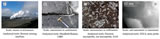 Figure 1
Comparison of geoanalytical scale. (A) Halemaumau crater, Kilauea, Hawaii. Photo by Molly McCanta. (B) Lava flow features, Kilauea. Photo by Nathan Bridges. (C) Photomicrograph of basaltic magma from Kilauea Iki lava lake. Photo by Molly McCanta. (D) Scanning transmission electron microscopy–electron energy loss spectroscopy (STEM-EELS) large grayscale high-angle dark field image of basaltic glass. Brighter areas show where iron is concentrated; bottom left corner shows the sample edge. LIBS—laser-induced breakdown spectroscopy; XAS—X-ray absorption spectroscopy.
This paper thus explores sampling strategies that result in the most accurate returned bulk rock properties from varying scales of measurements, rock types, textures, and analytical instruments. Rock characteristics (mineral and melt constituents, grain size) and analytical conditions (beam size, analysis location, number of analyses) are varied to study errors propagated onto bulk rock compositions. The results define the number of analyses required to get reproducible bulk rock compositions in lab and field applications. These are broadly relevant to any type of microanalysis, and also to sampling at field scales, where the ratio of hand sampling size to outcrop/formation scale heterogeneities is relevant.
Methodology
Grain size, beam size, phase assemblage, and phase composition are varied using a computer model to determine potential effects on the accuracy of bulk rock measurements. The modeling program returns mineral and oxide percentages along with standard deviations of the bulk composition represented by the average of the chosen analyses, which are randomly located. The model is built around a 2-D 1000 × 1000 pixel image. Applications to Mars exploration along with user input parameters are given in McCanta et al. (2013), and the model itself is available at www.mtholyoke.edu/~pdobosh/libssim/lasersimR5.html.
--------
1 GSA Data Repository Item 2017081, Table S1 (measured vs. calculated bulk compositions), is online at www.geosociety.org/datarepository/2017/. Questions? Please email gsatoday@geosociety.org.
Results
Accuracies of bulk compositions for multiple rock types, melt compositions, and beam conditions were calculated as a function of grain size, beam size, and sampling density. Grain size here refers to either mineral size in a crystalline rock or ionic radius of an atom within either a crystallographic matrix (mineral) or a randomly distributed amorphous matrix (melt).
Crystalline Rocks
To evaluate size ratio effects in crystalline rocks, basalt and dacite compositions from Mt. Shasta, California, USA, were used as program inputs. These natural island arc samples are fully crystallized, making it difficult to obtain a bulk composition as discussed above. Experimental work (Baker et al., 1994; McCanta et al., 2007) reproduced the melt-crystal assemblages, allowing bulk rock composition to be estimated and compared with model results. Variable grain sizes (Figs. 2A–2C), beam sizes, and sampling densities were studied (see GSA Data Repository1 Table S1). For each sampling density (10, 50, or 100 locations), three data sets are shown: grain size << beam size (ratio = 0.25), grain size = beam size (ratio = 1.0), and grain size >> beam size (ratio = 2.5). Precision values, represented by relative standard deviation (RSD), are given in Table 1.
 Figure 2
(A–C): Modeled basaltic “rocks” of varying grain size: red—glass, blue—olivine, purple—plagioclase, and pink—augite. Black squares are the sampling areas (50). Grain size relative to beam size increases to the right; beam size remains constant at 40 pixels. (A) Grain size = 10 pixels. (B) Grain size = 50 pixels. (C) Grain size = 150 pixels. (D–F): Comparison of true versus calculated bulk composition as grain size increases relative to beam size, with grain size < beam size (0.25), grain size ≈ beam size (1.25), and grain size > beam size (2.5). The solid line denotes where grain size and beam size are of equal size. Dashed lines represent the true electron probe microanalysis–determined bulk composition. Circles are the calculated values. (D) MgO. (E) Al2O3. (F) CaO.
 Table 1.
Precision of bulk composition data
Single Phase Systems
If only a single phase is present, then a reliable bulk composition requires few analyses, given the reasonable expectation that analytical precision is as good or better than accuracy. In our model results, six spot analyses are generally enough to generate a statistically significant bulk composition and account for minor heterogeneities; this number varies slightly with the relative precision and accuracy of each analytical method. These results apply to chemical measurements in glasses or homogeneous single crystals with sizes larger than the beam.
Grain Size
The presence of multiple phases introduces complications to sampling protocols and forces consideration of the grain-size to beam-size ratio. When grain size is small relative to the beam (ratio = 0.25; Fig. 2A), a single analysis likely samples a nearly representative portion of the assemblage, and may include all phases in the rock in their true proportions. Therefore, archetypal bulk compositions are returned when the sample grain size << beam size (Supplementary Table [see footnote 1]). As grain and beam size converge (grain size = beam size), calculated bulk compositions decrease in precision (Table 1). When grain size >> beam size (ratio = 2.5), it becomes unlikely that any microanalysis will sample all phases in a rock in correct proportions. In such cases, returned wt% oxide values do not accurately represent the bulk rock (Supplementary Table; Figs. 2D–2F), and the RSDs associated with such analyses are so large as to render them meaningless (Table 1).
Phase Assemblage
Although grain size is a significant determining factor in producing accurate bulk compositions, the chemistry of constituent minerals and glasses in the phase assemblage may also play roles. If a single phase contains the majority of an element in a system, it will have a disproportionate effect on bulk composition if the size of that mineral is close to the beam size. In the Shasta basalt experiments, olivine is the major MgO host and therefore controls the bulk MgO content. As grain size increases relative to beam size, errors associated with predicted MgO content get larger at a much faster rate than those of the other oxides (Fig. 3) due to disproportionate undersampling of the coarse-grained olivine. Other oxides in this basalt (CaO, Al2O3, SiO2) do not show similar behavior (Fig. 3). They occur in comparable amounts among all mineral phases (plagioclase, augite, glass), so representative sampling of them is not as critical to returning the true bulk rock composition.
 Figure 3
Comparison of influence of phase assemblage on the precision of the bulk analysis. Precision = percentage of the oxide value represented by the relative standard deviation (RSD*100). Elements that occur dominantly in one phase are more affected as grain size increases relative to beam size because they are more likely to be undersampled.
Number and Placement of Analysis Spots
From a statistical viewpoint, minerals in rocks can be viewed as randomly distributed unless there is textural evidence to the contrary (Figs. 2A–2C). As the number of analyses increases, calculated bulk composition gets closer to the true bulk value (Figs. 4A–4C; Supplementary Table). Analytical precision increases with sampling density as well, especially for minor elements or those concentrated in a single phase (i.e., MgO as noted above) (Table 1). In our modeled rocks, ~6–10 analyses are necessary for calculated bulk composition to fall within a 1σ error envelope of the real composition for most fine-grained samples (grain size < beam size) (Figs. 4A–4C). This is definitely not the case for coarse-grained samples (beam size > grain size; Fig. 4D), where sampling of even 100 locations does not reproduce calculated bulk compositions within the 1σ error envelope (Table 1).
 Figure 4
Comparison of sampling number with modeled bulk compositions. Solid line represents grain size << beam size; dotted line represents grain size >> beam size; dashed line is the true electron probe microanalysis oxide value. Modeled and true bulk values are approached within ~10 analyses for fine-grained samples (solid line) with larger beam spot sizes. Significantly more analyses are needed when the sample is coarse-grained (dotted line). (A) Al2O3. (B) FeO. (C) MgO. (D) Gore Mountain garnet outcrop. Circles represent the 1.5 cm diameter of possible Raman or laser-induced breakdown spectroscopy analytical dimensions. Note the difficulty in sampling a representative bulk composition even at these relatively large analytical sizes in a coarse-grained material. For comparison, with a 2 µm diameter beam size, 7,500 electron probe microanalysis or X-ray absorption spectroscopy spots would fit the diameter of each individual circle; for a 0.2 nm diameter beam size, 75,000,000 electron energy loss spectroscopy spots would fit the diameter of each individual circle.
Melt Properties
Geologists are increasingly investigating chemical phenomena that occur at smaller scales than the routine 1 μm EPMA measurement, such as measurement of iron redox state by X-ray absorption spectroscopy (XAS: spot size = 1000–5000 nm) and STEM-EELS (spot size = 0.1–0.2 nm). To illustrate the resulting issues of scale, we calculated Fe3+/Fe2+ ratios for a basaltic melt (BAS-2; Dyar et al., 2016) homogenized under oxidizing conditions. To simulate STEM-EELS measurements, a beam/sample order size ratio of 0.1 was used (beam size = 10 pixels; order size = 100 pixels; Fig. 5A). Here “order” reflects the extent of short- or long-range ordering in the glass/melt, which is unknown. For XAS measurements a beam/order size ratio of 950 was used (beam size = 950 pixels; ordering size = 1 pixel; Fig. 5B) because our model has maximum beam size of 1000 that results in full sample coverage.
 Figure 5
Modeled basaltic “melts.” Black squares are the sampling areas (20). (A) Electron energy loss spectroscopy measurements: beam/order size ratio = 0.1 (beam size = 10 pixels; order size = 100 pixels). (B) X-ray absorption spectroscopy measurements: beam/order size ratio = 950 (beam size = 950 pixels; order size = 1 pixel).
Beam Dimensions
Even when grain size is small, as in either crystallographic dimensions of a mineral or short range order in melts, variations in analytical spot size also result in sampling challenges. For example, the redox state of a melt (glass) can be calculated from its Fe3+/ΣFe ratio (e.g., Kilinc et al., 1983; Kress and Carmichael, 1991). Measured Fe3+ concentration must be representative of the bulk system to be interpretable. Our model simulates truly random melts (Figs. 5A and 5B), but natural silicate glasses may exhibit short range ordering on ~1–2 nm scales (e.g., Mysen and Richet, 2005). If beam size is much smaller than the short range ordering in the melt (e.g., STEM-EELS), a single analysis may sample only one atom (Fig. 5A), generating no representative information on the redox state of the bulk system (Table 2). Multiple analyses with this 0.1 beam/order ratio may never actually sample all of the elements present (Fig. 5A). Even with an impractically large number of analyses per single sample (n = 50), true bulk glass redox ratio is elusive (Table 2). Oxidation state of the sample cannot be quantified accurately without excessively large numbers of analyses.
When analytical beam size is several orders of magnitude greater than the short range order in the melt (e.g., XAS), a single analysis will sample a large, nearly representative number of atoms (Fig. 5B), and the calculated redox value approaches that of the true value (Table 2). Multiple analyses are still required to adequately cover the sample area and reduce standard deviations, but they do not significantly improve the match to the actual data (Table 2). The apparent decrease in the precision of the Fe2O3/FeO ratio with more analyses observed in Table 2 is an artifact of the model dimensions; when a single analysis covers nearly the whole sampling area, multiple analyses lead to increased analytical overlap, resulting in oversampling of the minor elements. This would not occur in a natural sample of near “infinite” dimension.
 Table 2.
Accuracy of melt redox compositions
Discussion
Using spot analyses to return representative data on a bulk sample thus requires consideration of several issues: the mineralogy or scale of ordering in a glass, texture (phase heterogeneity) of the target rock, distribution of textural features within each target, sampling size of the analytical instrument used, and sampling strategy employed (Fig. 6).
 Figure 6
Comparison of the number of analyses required for reproducible bulk compositional data as a function of the scale of sample to measurement heterogeneity (upper). The same plot is used to indicate where various analytical techniques and common geological samples might intersect (lower). STEM-EELS—scanning transmission electron microscopy–electron energy loss spectroscopy; XAS—X-ray absorption spectroscopy; LIBS—laser-induced breakdown spectroscopy; EPMA—electron probe microanalysis.
Target Rock Type
It is intuitive to understand how a beam that samples the maximum number of grains in proportions representative of the entire rock will yield optimal results. In coarser-grained rocks with varying abundances of minerals in their modes, sampling strategy becomes critical; it is very important that the phase assemblage be sampled proportionately. This may require plotting out sampling grids prior to analysis or point-counting phases on an outcrop to determine the major phenocryst concentration. In truly coarse-grained rocks (i.e., Fig. 4D), obtaining bulk compositions from smaller scale analyses is simply not feasible. However, in such samples individual mineral compositions may be representatively sampled, although fine-scale zonation might be obscured.
Sampling strategy is also critically important when the analytical instrument has a sampling size much smaller than the crystallinity or long-range ordering of the phase. As modern instrument resolution continues to increase, understanding of sampling strategy will become even more critically important.
It is less obvious that relative chemistries of the individual phases being studied are important; if even one phase has dramatically different elemental abundances over the other(s), then a larger number of analyses will be needed to represent the bulk. On the other hand, an ultramafic rock composed solely of olivine and pyroxenes might have much less elemental variability among phases, and thus require fewer analyses to be representative.
Distribution of Analysis Spots
Our model assigns sample locations randomly to prevent systematic sampling bias. In the field or in most microanalyses, analytical spots are chosen by the operator. Therefore, the distribution of sampling points must be strategically selected to minimize both the number needed and the sampling bias (Fig. 6). This can be accomplished in one of two ways: analyze a large number of truly randomly selected points, or estimate the mineral mode and apportion analysis locations to represent each one appropriately (i.e., Chayes, 1956). The former is generally far easier than the latter, with the modal analysis method presenting the additional potential issue of assuming a 2D surface mode characterization represents a 3D rock sample. New software for quantitative EPMA mapping, which can provide full compositional quantification of each image pixel (e.g., Carpenter et al., 2013; Carpenter, 2016), may reduce sampling bias and better account for geochemical heterogeneity.
For rocks with distinct foliation, lineation, grain preferred orientation, or layering, sampling strategy becomes even more important; in these samples, an accurate bulk rock composition may not be meaningful. For example, if a rock is layered, sampling traverses should cross-cut bedding planes with a sampling interval smaller than the layering interval to ensure proportional representation of each layer. Alternatively, traverses that probe a single layer laterally may be extremely useful, especially if multiple layers are similarly studied for contrast.
Number of Analyses Needed
Several sampling strategies can ensure quality analyses with reproducible results (Fig. 6). First, the larger the ratio between grain and beam size, the more analyses are required. For grain sizes << beam size, 6–10 analyses produce a statistically meaningful result as long as the phases present are sampled proportionally (Figs. 4A–4C) and measurement accuracy is appropriate. When the scale of grain size or the extent of ordering is close to or exceeds beam size (Fig. 4D), significantly more analyses are needed (up to 1000) to generate reproducible bulk compositional data. When more than one phase is present, analysis locations must be designed to represent all phases in the rock proportionately if a true bulk rock analysis is desired.
Conclusions
Our models show quantitatively what is intuitively obvious: heterogeneous rocks with coarse grain sizes present great challenges when obtaining bulk analyses. Care must be taken both when choosing randomly distributed analytical points and when interpreting data from instruments with different sampling volumes (Fig. 6). Moreover, rocks with visible texture (layering, phenocrysts, etc.) must be carefully sampled (if bulk compositions are needed) to ensure that analysis locations are proportionally representative of all textures present (Fig. 6). Additionally, the ratio of sample size to analytical size needs to be considered, especially as modern instruments resolve increasingly small analytical volumes. The concept of a “bulk analysis” likely needs to be revised for each system, following the methods provided in this study (Fig. 6).
Acknowledgments
We acknowledge funding from NSF grants EAR-1219850 (MCM) and EAR-1219761 (MDD). Reviews from two anonymous reviewers were thorough and strengthened this paper.
References Cited
- Asimow, P.D., 2000, Melting of the mantle, in Sigurdsson, H., Houghton, B., McNutt, S.R., Rymer, H., and Stix, S., eds., Encyclopedia of Volcanoes: San Diego, Academic Press, p. 55–68.
- Baker, M.B., Grove, T.L., and Price, R., 1994, Primitive basalts and andesites from the Mt. Shasta region, N. California: Products of varying melt fraction and water content: Contributions to Mineralogy and Petrology, v. 118, p. 111–129, doi:10.1007/BF01052863.
- Basaltic Volcanism Study Project, 1981, Basaltic Volcanism on the Terrestrial Planets: New York, Pergamon Press Inc., 1286 p.
- Bowen, N.L., 1928, The Evolution of the Igneous Rocks: Princeton, New Jersey, Princeton University Press, 334 p.
- Bucher, K., and Frey, M., 2002, Petrogenesis of Metamorphic Rocks: Heidelberg, Springer-Verlag, 440 p., doi: 10.1007/978-3-662-04914-3.
- Carpenter, P.K., 2016, Compositional stage mapping by EPMA and micro-XRF: Microscopy and Microanalysis, v. 22, p. 94–95, doi: 10.1017/S143192761600132X.
- Carpenter, P.K., North, S.N., Jolliff, B.L., and Donovan, J.J., 2013, EPMA quantitative compositional mapping and analysis of lunar samples: Lunar and Planetary Institute, 44th Lunar and Planetary Science Conference, abstract 1827.
- Chayes, F., 1956, Petrographic Modal Analysis: An Elementary Statistical Appraisal: New York, John Wiley & Sons, 113 p.
- Cox, K.G., Bell, J.D., and Pankhurst, R.J., 1979, The Interpretation of Igneous Rocks: London, George Allen & Unwin, 450 p., doi:10.1007/978-94-017-3373-1.
- Daly, R.A., 1933, Igneous Rocks and the Depths of the Earth: New York, Hafner Publishing Company, 598 p.
- Dyar, M.D., McCanta, M.C., Breves, E., Carey, C.J., and Lanzirotti, A., 2016, Accurate predictions of iron redox state in silicate glasses: A multivariate approach using X-ray absorption spectroscopy: American Mineralogist, v. 101, p. 744–747.
- Garvie, L.A.J., and Buseck, P.R., 1998, Ratios of ferrous to ferric iron from nanometre-sized areas in minerals: Nature, v. 396, p. 667–670, doi:10.1038/25334.
- Kelly, T.F., and Larson, D.J., 2012, Atom Probe Tomography 2012: Annual Review of Materials Research, v. 42, p. 1–31, doi:10.1146/annurev-matsci-070511-155007.
- Kilinc, A., Carmichael, I.S.E., Rivers, M.L., and Sack, R.O., 1983, The ferrous-ferric ratio of natural silicate liquids equilibrated in air: Contributions to Mineralogy and Petrology, v. 83, p. 136–140.
- Kress, V., and Carmichael I.S.E., 1991, The compressibility of silicate liquids containing Fe2O3 and the effect of composition, temperature, oxygen fugacity, and pressure on their redox states: Contributions to Mineralogy and Petrology, v. 108, p. 82–92.
- Martin, J.W., 2003, The Local Chemical Analysis of Materials: London, Elsevier, 234 p.
- McCanta, M.C., Rutherford, M.J., and Hammer, J.E., 2007, Pre-eruptive and syn-eruptive conditions in the Black Butte, California dacite: Insight into crystallization kinetics in a silicic magma system: Journal of Volcanology and Geothermal Research, v. 160, p. 263–284, doi:10.1016/j.jvolgeores.2006.10.004.
- McCanta, M.C., Dobosh, P.A., Dyar, M.D., and Newson, H.E., 2013, Testing the veracity of LIBS analyses on Mars using the LIBSSIM program: Planetary and Space Science, v. 81, p. 48–54, doi:10.1016/j.pss.2013.03.004.
- Mysen, B.O., and Richet, P., 2005, Silicate Glasses and Melts: Properties and Structure: San Diego, Elsevier Inc., 560 p.
- Nutman, A.P., Mojzsis, S.J., and Friend, C.R.L., 1997, Recognition of ≥3850 Ma water-lain sediments in West Greenland and their significance for the early Archaean Earth: Geochimica et Cosmochimica Acta, v. 61, p. 2475–2484, doi:10.1016/S0016-7037(97)00097-5.
- Philpotts, A.R., and Ague, J., 2009, Principles of Igneous and Metamorphic Petrology: Cambridge, Cambridge University Press, 686 p., doi:10.1017/CBO9780511813429.
- Potts, P.J., Bowles, J.F.W., Reed, S.J.B., and Cave, M.R., editors, 1995, Microprobe Techniques in the Earth Sciences: London, Chapman & Hall, 430 p., doi: 10.1007/978-1-4615-2053-5.
- Powell, R., Holland, T.J.B., and Worley, B., 1998, Calculating phase diagrams involving solid solutions via non-linear equations, with examples using THERMOCALC: Journal of Metamorphic Geology, v. 16, p. 577–588, doi:10.1111/j.1525-1314.1998.00157.x.
- Valley, J.W., Reinhard, D.A., Cavosie, A.J., Ushikubo, T., Lawrence, D.F., Larson, D.J., Kelly, T.F., Snoeyenbos, D.R., and Strickland, A., 2015, Nano- and micro-geochronology in Hadean and Archean zircons by atom-probe tomography and SIMS: New tools for old minerals: The American Mineralogist, v. 100, p. 1355–1377, doi:10.2138/am-2015-5134.
- van Aken, P., and Liebscher, B., 2002, Quantification of ferrous/ferric ratios in minerals: new evaluation schemes of Fe L23 electron energy-loss near-edge spectra: Physics and Chemistry of Minerals, v. 29, p. 188–200, doi:10.1007/s00269-001-0222-6.
- Yoder, H.S., Jr., and Tilley, C.E., 1962, Origin of basaltic magmas: An experimental study of natural and synthetic rock systems: Journal of Petrology, v. 3, p. 342–532, doi:10.1093/petrology/3.3.342.