Full Text View
Volume 23 Issue 4 (April/May 2013)
GSA Today
![]()
Article, pp. 60–61 | Abstract | PDF (92KB)
 |
| Table of Contents |
|---|
| Search GoogleScholar for Search GSA Today |
GROUNDWORK:
How good do natural hazard assessments need to be?
1 Earth and Planetary Sciences, Northwestern University, Evanston, Illinois 60208, USA
2 Applied Mathematics, Brown University, Providence, Rhode Island 02912, USA
In trying to mitigate natural hazards, society plays a high-stakes game against nature. Often nature surprises us when an earthquake, hurricane, or flood is bigger or has greater effects than expected from detailed natural hazard assessments. In other cases, nature outsmarts us, doing great damage despite expensive mitigation measures.
These difficulties are illustrated by the March 2011 earthquake off Japan’s Tohoku coast. The earthquake was much larger than anticipated from hazard maps and generated a tsunami much larger than anticipated, which overtopped coastal defenses, causing more than 15,000 deaths and US$210 billion damage. Similar situations occur in predicting earthquake ground shaking (Stein et al., 2012), river floods (Merz, 2012), and other hazards (Pollack, 2003; Pilkey and Pilkey-Jarvis, 2007).
* Email:
**Jerome Stein, Professor Emeritus of Economics at Brown University, died on 8 February 2013. During a long illness, he coauthored a series of papers and a forthcoming book on integrating geosciences and economics in natural hazard mitigation.
Manuscript received 17 Nov. 2012; accepted 7 Jan. 2013
doi: 10.1130/GSATG167GW.1
Society faces the challenge of choosing mitigation strategies, given that assessments of potential hazard have large uncertainties. This challenge is similar to that in national defense, involving choosing among expensive weapons and strategies to deal with poorly known future threats. Like defense planners, hazard planners must decide how much is enough (Enthoven and Smith, 1971; Goda and Hong, 2006).
We explore choosing strategies using a simple model comparing the costs and benefits of mitigation options (Stein and Stein, 2012). For example, given the damage to New York City by the storm surge from Hurricane Sandy, options under consideration range from continuing to do little through intermediate strategies like providing doors to keep water out of vulnerable tunnels to building barriers to keep the surge out of rivers. Progressively more extensive mitigation measures cost more but are expected to produce increasing reduction of losses in future hurricanes.
In our model, we denote the cost of mitigation as C(n), where n is a measure of mitigation. The scale of a natural event is parameterized by h, such as the height of a storm surge, an earthquake’s magnitude, or the level of the resulting ground shaking. The predicted annual economic loss, L(h,n) increases with h and decreases with n. The annual probability of an event h is p(h), so the present value of the expected loss is
![]() (1)
(1)
the sum of losses from different events weighted by their probabilities. The hazard is described by p(h), the occurrence of events of a certain size, and Q(n) reflects the risk, which depends on the mitigation level n. Because the dates of future events are unknown, L(h,n) is the expected average direct and indirect annual loss.
A sum of money S invested today at interest rate i will be worth S(1 + i)t at a future time t, so the present value of a sum S at a future time t is the inverse, S/(1 + i)t.Thus, we scale the future losses to their present value using the sum over T years
![]() (2)
(2)
for large T. For interest rate i = 0.05, DT = 15.4for 30years and 19.8 for 100 years. For long times, 1/i gives D = 20, essentially the same as for 100 years. Given the long lives of mitigation measures, 1/i is appropriate.
The optimum level of mitigation n* minimizes the total cost K(n), the sum of the expected loss and mitigation cost
![]() (3)
(3)
The “U”shaped K(n) curve illustrates the tradeoff between mitigation and loss (Fig. 1A). For no mitigation, n = 0, the total cost K(0) equals the expected loss Q(0). Initial levels of mitigation reduce the expected loss by more than their cost, so K(n) decreases to a minimum at the optimum. K(n) is steepest for n = 0 and flattens as it approaches the optimum, showing the decreasing marginal return on investment in mitigation. Relative to the optimum, less mitigation decreases mitigation costs but increases the expected damage and thus total cost, so it makes sense to invest more in mitigation. Conversely, more mitigation than the optimum gives less expected damage but at higher total cost, so the additional resources required could do more good if invested otherwise.
The optimum can be viewed using the derivatives of the functions, which for simplicity are shown as linear near the optimum (Fig. 1B). Because increasingly high levels of mitigation cost more, the marginal cost C′(n) increases with n. Conversely, −Q′(n), the reduced loss from additional mitigation, decreases. The lines intersect at the optimum, where
![]() (4)
(4)
|
(A) Comparison of total cost curves for two estimated hazard levels. For each, the optimal mitigation level, n*, minimizes the total cost, the sum of expected loss and mitigation cost. (B) In terms of derivatives, n* occurs when the reduced loss −Q′(n) equals the incremental mitigation cost C′(n). If the hazard is assumed to be described by one curve but actually described by the other, the assumed optimal mitigation level causes non-optimal mitigation, and thus excess expected loss and/or excess mitigation cost. However, so long as the total cost is below the loss for no mitigation (dashed line), this non-optimal mitigation is better than none. Thus an inaccurate hazard estimate is useful as long as it is not too much of an overestimate. |
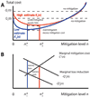 Figure 1
Although over-mitigation and under-mitigation are less efficient uses of resources than the optimum, a range of non-optimal solutions is still better than no mitigation. So long as K(n) is below the dashed line Q(0), the total cost is less than expected from doing no mitigation. The curve and line intersect again when
![]() (5)
(5)
which is where the benefit to society, the reduced loss compared to doing no mitigation Q(0) − Q(n),equals the mitigation cost C(n). Higher levels of mitigation cost more than their benefit and thus are worse than no mitigation.
Because our ability to assess natural hazards is limited, we consider a range of total cost curves between K1(n) and K2(n), corresponding to high and low estimates of the hazard. These start at different values, representing the expected loss without mitigation, and converge for high levels of mitigation as the mitigation costs exceed the expected loss.
In the limiting cases, the hazard is assumed to be described by one curve but is actually described by the other. As a result, the optimal mitigation level chosen for the assumed curve gives rise to non-optimal mitigation, shown by the corresponding point on the other curve. Assuming low hazard when higher hazard is appropriate causes under-mitigation and thus excess expected loss. Assuming high hazard when lower hazard is appropriate causes over-mitigation and thus excess mitigation cost. However, so long as this point is below the dashed linefor the correct curve, the total cost is less than expected from doing no mitigation.
Given the range of hazard estimates, decision theory under deep uncertainty (Cox, 2012) suggests that society should choose an estimate between them. The resulting curve lies between the two curves and thus has a minimum between n1* and n2*. Relative to the actual but unknown optimum, the resulting mitigation is likely non-optimal but perhaps not unduly so. Moreover, so long as the total cost is below the actual loss for no mitigation, this non-optimal mitigation is better than no mitigation.
Hazard and loss modeling are subject to uncertainties with various causes. In addition to the uncertainty in the probability of future events, uncertainty in the expected loss results from uncertainty in specifically what occurs and how effective mitigation measures will be in reducing loss. For example, for an earthquake of a given magnitude, uncertainty arises in predicting both the ground shaking and the resulting damage. These uncertainties are typically characterized in overlapping terms, into epistemic uncertainties due to systematic errors and aleatory (aleae is Latin for dice) uncertainties due to random variability about assumed means. In our formulation, the different cost curves can be viewed as illustrating epistemic uncertainties. Aleatory uncertainties can be viewed as variations about a curve and incorporated via a term that can also include the effects of risk aversion, which describes the extent to which we place greater weight on avoiding loss (Stein and Stein, 2012).
Because the “U” curves are the sum of loss and mitigation costs, uncertainties in loss estimation have the same effect as those in hazard estimation. Hence, the two cases can be viewed as high and low estimates of the loss for an assumed hazard. In reality, the range would reflect the combined uncertainty in hazard and loss estimates.
The analysis illustrates two crucial points. First, a non-optimal mitigation strategy—which is usually the case because the decisions are made politically rather than via economic analysis—still does more good than doing nothing as long as it is not so extreme that the mitigation costs exceed the benefit of reduced losses. Second, inaccurate hazard and loss estimates are still useful as long as they are not too much of an overestimate. Given that most natural hazards assessments and estimates of the resulting losses have large uncertainties, it is encouraging that any estimate that does not greatly overestimate the hazard and loss leads to a mitigation strategy that is better than doing nothing.
Acknowledgment
We thank the U.S. Geological Survey John Wesley Powell Center for Analysis and Synthesis for hosting a working group that inspired this work, and John Adams, John Geissman, Tom Holzer, Ross Stein, David Wald, and an anonymous reviewer for insightful comments.
References Cited
- Cox, L.A., Jr., 2012, Confronting deep uncertainties in risk analysis: Risk Analysis, v. 32, no. 10, p. 1607–1629, doi: 10.1111/j.1539-6924.2012.01792.x.
- Enthoven, A., and Smith, K., 1971, How Much is Enough? Shaping the Defense Program 1961–1969: Santa Monica, California, Rand Corporation, 349 p.
- Goda, K., and Hong, H.P., 2006, Optimum seismic design considering risk attitude, societal tolerable risk level and life quality criterion: Journal of Structural Engineering, v. 132, p. 2027–2035.
- Merz, B., 2012, Role and responsibility of geoscientists for mitigation of natural disasters: European Geosciences Union Assembly, Vienna.
- Pilkey, O.H., and Pilkey-Jarvis, L., 2007, Useless Arithmetic: Why Environmental Scientists Cant Predict the Future: New York, Columbia University Press, 248 p.
- Pollack, H.N., 2003, Uncertain Science Uncertain World: Cambridge, UK, Cambridge University Press, 256 p.
- Stein, J.L., and Stein, S., 2012, Rebuilding Tohoku: A geophysical and economic framework for hazard mitigation, GSA Today, v. 22, no. 10, p. 42–44, doi: 10.1130/GSATG154GW.1.
- Stein, S., Geller, R.J., and Liu, M., 2012, Why earthquake hazard maps often fail and what to do about it: Tectonophysics, v. 562–563, p. 1–25.