
Full Text View
Volume 21 Issue 12 (December 2011)
GSA Today
![]()
Article, pp. 4-10 | Abstract | PDF (3.1MB)
Unique geologic insights from “non-unique” gravity and magnetic interpretation
Abstract
Interpretation of gravity and magnetic anomalies is mathematically non-unique because multiple theoretical solutions are always possible. The rigorous mathematical label of “non-uniqueness” can lead to the erroneous impression that no single interpretation is better in a geologic sense than any other. The purpose of this article is to present a practical perspective on the theoretical non-uniqueness of potential-field interpretation in geology. There are multiple ways to approach and constrain potential-field studies to produce significant, robust, and definitive results.
The “non-uniqueness” of potential-field studies is closely related to the more general topic of scientific uncertainty in the Earth sciences and beyond. Nearly all results in the Earth sciences are subject to significant uncertainty because problems are generally addressed with incomplete and imprecise data. The increasing need to combine results from multiple disciplines into integrated solutions in order to address complex global issues requires special attention to the appreciation and communication of uncertainty in geologic interpretation.
*E-mails: ;
Manuscript received 18 Aug. 2011; accepted 3 Oct. 2011.
DOI: 10.1130/G136A.1
Introduction
Potential theory traces its long roots back to Isaac Newton’s 1687 Universal Law of Gravitation and Pierre Laplace’s 1770 paper on differential equations. In mathematical terms, potential theory describes functions that satisfy a basic differential equation known as Laplace’s equation. These functions include those describing natural forces that decrease with distance from their causative sources (e.g., gravity and magnetic fields), as well as electrical fields, steady-state heat flow, some fluid flow, and the behavior of elastic solids. Green (1828) is evidently the first to apply the term “potential” to the mathematics of this set of phenomena. Parker (1973) eloquently summarizes the non-uniqueness of potential fields in the context of the Earth sciences. For more detail on the theoretical underpinnings of gravity and magnetic applications, see Blakely (1995).
The rich mathematics of potential-field theory provides the basis for a variety of tools to analyze and explain gravity and magnetic anomalies. For example, Fourier domain filters allow us to transform and decompose potential-field data and facilitate map-based interpretations. Modern software and computers allow us to calculate the gravity or magnetic effects of modeled geological formations and test these models against observed data. And powerful tools and techniques continue to be developed for calculating specific physical properties or other structural characteristics directly from gravity and/or magnetic measurements.
A basic illustration of the non-uniqueness of unconstrained potential-field interpretation is the construction of a set of discrete bodies, each of which yields the same calculated anomaly. Figure 1 (modified from figure 4.18 in Sleep and Fujita, 1997) shows a stack of carefully crafted density bodies, ranging from a broadly tapered shallow source to a compact deeper source, each producing the same bell-shaped anomaly. This same figure illustrates another oft-quoted property of potential-field solutions: Changing the sign of the density contrast on one of these hypothetical bodies produces an equal and opposite anomaly to one of the other bodies; thus, we can add any number of these specially designed bodies with alternating signs and not change the total calculated anomaly.
|
Results of two-dimensional calculation of the gravity effect of the source bodies (A, B, and C) depicted in the cross section view (bottom panel). When the smooth theoretical shape of each is used, the resulting calculated anomaly is identical in all three cases, as depicted by the smooth dotted line labeled “A, B, or C theoretical.” However, when the source bodies include some irregularity in their shape, as expected in the real world, the calculated gravity anomaly will differ from the smooth theoretical result (as shown by the “B actual” and “C actual” curves). The difference between the anomalies caused by the theoretical and actual shapes is shown by the “error” curves in the top panel. These differences will depend on the depth to source bodies as illustrated by the broad wavelength for the B error curve and the narrower wavelength for the C error curve. |
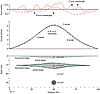 Figure 1
While these theoretical diagrams are interesting for learning about the mathematics of potential fields, they are not particularly relevant to real-world applications. What are the chances that nature will produce two perfectly cancelling anomaly sources? Real-world anomaly sources are unlikely to have an ideal shape and perfect homogeneity. As a result, shallow source bodies (like body “C” in Fig. 1) will produce, in addition to the broad anomaly, short wavelength features that correlate with the natural and expected irregularities of any true geologic body. A deeper body (like body “A” in Fig. 1) will produce a smoothly varying anomaly because the short-wavelength attributes of the anomaly are naturally damped with distance. Thus, the additional information provided in the real world allows us to intelligently decide on the likely depth of the body, regardless of the fact that infinitely many models may be constructed to fit the data mathematically. In the next two sections, we follow up on this idea of practical versus theoretical non-uniqueness; we argue that (1) many unique and important conclusions can be drawn directly from potential-field data, and (2) even basic geologic constraints provide sufficient a priori knowledge to allow for significant results.
Unique Gravity and Magnetic Results with Little or No A Priori Information
A number of fundamentally unique results arise directly from analysis of gravity and magnetic data. It is possible, for example, to calculate the total anomalous mass causing a gravity anomaly, and this has application to a number of practical problems. A basin filled with sediments causes a gravity low because of the contrast between low-density sediments that fill the basin and higher density rocks that surround it. The total mass deficit of the basin is given unequivocally by integration of the gravity anomaly across the entire anomaly. That calculation requires no knowledge of the actual densities. We can extend our knowledge if we can determine reasonable densities from geologic arguments and rock property analysis. In particular, knowing the total mass deficit and assuming a maximum density contrast between sediments and rocks provides the minimum volume of the basin, a useful measure of erosion and mass transport. Another potential-field technique that yields unique results with few a priori assumptions is the Nettleton method for determination of average density (Nettleton, 1971). Using this technique, it is possible to estimate the average density of topography by selecting a Bouguer gravity reduction density that minimizes the correlation between topography and Bouguer gravity anomaly.
Another unique result from gravity and magnetic analysis is the use of maximum gradients to map physical property boundaries and trends (Cordell, 1978; Blakely and Simpson, 1986; Grauch and Cordell, 1987). The directionality, linearity, continuity, and many other attributes of physical boundaries are important structural and geological indicators. For example, many faults and fault zones have well-known gravity and magnetic expression (e.g., Langenheim et al., 2004; Jachens et al., 2002, Blakely et al., 2002; Saltus, 2007; Grauch et al., 2001). Tectonic boundaries also have prominent and distinctive gravity and magnetic expression (e.g., Lillie, 1999; Turcotte and Schubert, 2002), including the trends and amplitudes of anomalies.
In many cases, general estimates of potential-field sources can be derived directly from measured anomalies without appeal to specific assumptions about the source distribution. For example, a basic graphical technique (Peters, 1949) gives a reasonable estimate of depth to the top of a density or magnetic source. Similarly, limits on source depths can be found using relatively simple formulas (e.g., Bott and Smith, 1958; Smith, 1959). Many of these “rule of thumb” and other direct interpretation methods were developed in the early (i.e., pre-computer) period of modern geophysical exploration. More advanced depth estimation techniques (e.g., Phillips, 1979; Reid et al., 1990; Nabighian and Hansen, 2001; Phillips et al., 2007; Salem et al., 2008) are now available as computer codes and, in most cases, yield stable results when properly applied. Certain geometric constraints can produce unique results (e.g., Smith, 1961; Cordell, 1994). Parker and Heustis (1974) and Parker (1975) cover this topic well, including the introduction of the concept of “ideal bodies,” a way to derive certain fundamental source characteristics that are properties of all possible theoretical solutions.
Robust Potential-Field Results with Even Modest Amounts of A Priori Information
Even the most basic geologic constraints are often sufficient to yield specific, robust, and defendable potential-field interpretations. For example, the dip direction of a fault is determined directly by observing the form of the gravity anomaly step across the fault. The position of the midpoint of the step in gravity anomaly relative to the mapped surface trace of the fault indicates direction of dip (Fig. 2; inspired by fig. 4.19 in Sleep and Fujita, 1997). Another geologic example involves extension of geologic mapping from areas of outcrop into covered regions. In many cases the patterns of gravity and magnetic anomalies can be confidently associated with observed geologic units, and the continuation of these same patterns can be observed in adjacent covered regions (e.g., Jaques et al., 1997).
|
Cross section to illustrate unique interpretation of fault dip if surface trace of the fault is known. Midpoint of the step in gravity anomaly falls directly over fault trace for a vertical fault. If the midpoint is offset from the fault trace, it indicates the direction of fault dip. |
The point here is that interpretation of potential-field data, while mathematically non-unique, still provides practical information when a priori knowledge is blended into the solution. In fact, every credible potential-field interpretation does this. Call it a “geophysical bill of rights”: We hold certain truths to be self-evident—e.g., regional crustal density will never exceed 4000 kg/m3; rocks hotter than the Curie temperature (~580 °C) don’t produce significant magnetic anomalies; and seismic-reflection methods will see and constrain physical property boundaries. Applying these (and many other) constraints reduces the infinite set of answers to a smaller set of plausible ones. Interpreted solutions become increasingly constrained as additional information is included, such as geologic mapping, rock property measurements, and results from other geophysical methods.
Non-Uniqueness and Uncertainty in the Earth Sciences
While the “non-uniqueness” label is frequently associated with potential-field interpretations and results, it is worth noting that many broader aspects of geologic and geophysical interpretation are also subject to ambiguity. In fact, making interpretations from incomplete evidence is the rule rather than the exception in much of geology (Frodeman, 1995).
For example, in all but the most simple geologic settings even basic geologic mapping is “non-unique.” Send two different geologists into a complex region with poor outcrop and you will get two different geologic maps. In his erudite presidential address to GSA, Krauskopf (1968) discusses in great detail the difficulties of mapping ten plutons in the Sierra Nevada, emphasizing the complex considerations in choosing and defending geologically mappable units. Modern digital mapping and real-time capture of data in the field offer opportunities for quantifying mapping uncertainty and recording field interpretation choices (Jones et al., 2004), and computer methodologies have been created to approach the quantification of mapping uncertainty (e.g., Brodaric et al., 2004). Nevertheless, most published geologic maps contain significant uncertainties that can be difficult to estimate, particularly for non-geologists.
Interpretation of seismic data is also subject to ambiguity and “non-uniqueness” (e.g., Bond et al., 2007; Rankey and Mitchell, 2003). In seismic refraction, the unequivocal identification of seismic wave phases is often challenging, especially in complex and/or noisy settings. In seismic reflection, the identification and interpretation of geologic structure is subject to many judgment calls, and the process of migrating data from time to depth also depends on the experience and judgment of the practitioner. Seismic data are frequently “re-processed” to make iterative improvements and changes to interpretations—if the solution was unique, there would never be a need for reprocessing.
Examples of Robust Geological Insight from Gravity and Magnetic Analysis
One of the most fundamental examples of potential-field interpretation is the association of oceanic magnetic stripes with the concept of sea-floor spreading (e.g., Vine and Matthews, 1963; Vine, 1966) (Fig. 3). In this case, direct observation of the anomaly pattern is interpreted in terms of sea-floor spreading, the geomagnetic time scale, and the well-established concept of remanent magnetism. The patterns of the positive and negative anomaly “stripes” are correlated with the patterns of normal and reversed magnetic epochs in the geomagnetic time scale. The reliability of the interpretations is not affected by the mathematical non-uniqueness of potential-field interpretation.
|
The positive magnetic anomaly stripes are colored to match their association with the geomagnetic polarity time scale (redrawn from original by Vine, 1966). |
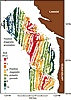 Figure 3
Another unambiguous application of potential-field interpretation is the use of gravity and/or magnetic maps to trace geologic units under surficial cover (e.g., dense vegetation and/or young sediments). In many cases, mapped lithologies have distinctive geophysical expression, and this can be firmly established by the spatial coincidence of outcrop with geophysical map patterns. These ties to lithology are strengthened by in situ measurement of physical properties to verify the suspected source of specific geophysical features (e.g., high densities measured on a mafic intrusion or reversed and normal polarity magnetic remanence measured on basaltic flows). Gettings (2002) (Fig. 4) shows the concealed continuation of a mapped suite of granitic to dioritic intrusions using data from an aeromagnetic survey in the Santa Cruz Valley, Arizona. Blakely et al. (2000, 2011) apply this idea to map rocks of the Columbia River Basalt series beneath adjacent surficial geology. There are many other formal and informal examples of this potential-field application; in fact, too many to cite here. This “pattern matching” approach is widely used, for example, in geologic mapping and exploration in places like Alaska (e.g., Werdon et al., 2004; Day et al., 2007), where much of the geology is concealed and logistics are expensive.
|
Mapped geology (A; simplified from Drewes, 1971) and magnetic anomalies (B) in Santa Cruz Valley, Arizona, USA (Gettings, 2002). High amplitude magnetic anomalies correlate with mapped intrusive rocks (e.g., anomalies labeled A, B, C, and D) and indicate the presence of additional intrusive rocks under sedimentary and volcanic cover (e.g., anomalies labeled 1, 2, and 3). See Gettings (2002) for additional detail; this figure is greatly simplified. |
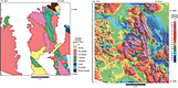 Figure 4
Another direct application of potential-field study is mapping of important geologic contacts, most notably faults, between exposures or other locations known from LiDAR or trenching. This is particularly important in regions of human disturbance, such as urban centers. As with much of potential-field analysis, there are examples of this approach at a wide range of scales. At the continental scale, Bischke et al. (1990) map the regional continuation of the Philippine fault system. Saltus (2007) shows the detailed location of the Tintina fault and uses the matching of distinctive anomalies transposed by the fault to deduce amount of fault movement. Blakely et al. (2002) (Fig. 5) use compiled aeromagnetic surveys to follow the Seattle fault under the heavily populated Puget Lowland from Bremerton east to Bellevue and beyond. The concept of using potential-field patterns for the mapping of geologic entities between known locations also applies to connecting seismically mapped structures between widely spaced seismic lines (e.g., Phillips, 1999).
|
Example of using magnetic anomalies to map subsurface lithologies. A, B, and C on top map indicate sinuous magnetic anomalies (positive, negative, and positive, respectively) above the hanging wall of the Seattle fault, Washington, USA. Analysis of these data lead to the interpretation shown in the lower map, where the sources of anomalies A, B, and C are interpreted as steeply dipping Miocene conglomerate, relatively nonmagnetic Oligocene sedimentary rocks, and Eocene volcanic rocks, respectively. Interpretation is constrained by geologic mapping, LiDAR surveys, and seismic-reflection interpretations. See Blakely et al. (2002) for details. |
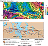 Figure 5
Examination and analysis of potential-field anomalies provides a powerful and direct way to choose between geologic scenarios; in many cases, geologic concepts can be tested and confidently rejected if they do not jibe with their geophysical implications. One can readily distinguish vertical tectonic models from lateral tectonic models in orogenic regions by simple examination of correlations between gravity and topography. Mountains with deep crustal roots (e.g., the Sierra Nevada in California) have distinctly different gravity expression from rootless mountains (e.g., ranges in Wyoming). For example, Saltus et al. (2001) rule out thin-skinned interpretation of the Copter Peak allochthon in the western Brooks Range by testing it against measured gravity and magnetic anomalies in conjunction with measured physical properties (density and magnetic susceptibility) of exposed mafic rocks.
In some cases, individual anomalies are sufficiently isolated and simple that they can be confidently modeled in detail. For example, Thompson and Robinson (1975) construct detailed models of the magnetic and gravity anomalies of the Twin Sisters Dunite in Washington state, and Burns (1983, 1985) models a portion of the Knik Arm magnetic anomaly (Cook Inlet, Alaska) by tying it to surface outcrop of Jurassic intrusives with high measured magnetic susceptibility. Even if a single specific solution is not possible, important bounds on solutions can frequently be established, as Blakely (1994) demonstrates, or key elements of the solution can be identified (e.g., shapes of sedimentary basins; Jachens and Moring, 1990; Saltus and Jachens, 1995).
DISCUSSION
Uncertainty is fundamental to the scientific endeavor. Every scientific conclusion is subject to review and is only as good as the assumptions and methodologies that went into it. Scientists construct working hypotheses, models, and experiments to test our understanding. If a model or hypothesis produces results that agree with data and experiment, we regard it as successful for the time being, recognizing it may ultimately fail and need to be corrected, updated, or abandoned in light of new discovery or understanding. The widely quoted (and variously attributed) maxim “all models are wrong, but some are useful” is an expression of the basic nature of science. In terms of uncertainty we could rephrase this maxim as “all models are uncertain, but some are better than others.”
The broader issue in potential fields, as in all science, is the effective and accurate communication of uncertainty (including aspects of non-uniqueness) in our interpretations (Frodeman, 1995; Bond et al., 2007). Indeed, the difficulties of dealing with uncertainty are a fundamental part of ordinary life and not confined to science or any other particular human endeavor (as Pollack, 2003, elegantly discusses). Earth scientists routinely deal with more uncertainty in interpretation than some other scientists because of the generally incomplete nature of our data sampling (Frodeman, 1995). The mathematical non-uniqueness of potential fields requires direct acknowledgment of uncertainty—perhaps more so than for other methods in the Earth sciences. As such, the study of potential-field interpretation provides fertile ground in which to explore the practical implications of theoretical uncertainty.
Many of the greatest scientific challenges of today span the traditional subdivisions of science. Climate change research, for example, spans Earth, atmospheric, and biological sciences and requires the combination of results from physics, chemistry, biology, geology, engineering, sociology, and economics. A key component to successful integrated science is the effective communication and mutual understanding of uncertainties arising in all of the component studies that feed into the ultimate integrated solution. But, it is also important to realize that the ultimate significance of a given result is not necessarily related to the relative certainty of that result. A partial solution or constraint to a fundamental problem may have greater significance than an exact solution to a trivial problem. And an effective integrated solution may encompass a wide range of uncertainties in the component results. To paraphrase Aristotle: The whole (integrated interpretation) is greater than the sum of its parts (methods and assumptions). And, we might add, the individual parts do not necessarily contribute equally to the sum.
SUMMARY
As career practitioners of potential-field interpretation, we feel that the theoretical non-uniqueness of potential-field interpretation creates possible confusion about the reliability of potential-field results. All credible potential-field studies judiciously incorporate a priori constraints such as physical property data, geologic mapping, or seismic interpretation to constructively limit the infinite theoretical universe of possible solutions. Furthermore, we feel that the general topic of “non-uniqueness” (and the closely related concepts of uncertainty and error analysis) in the Earth sciences (and indeed, science in general) deserves ongoing discussion and debate, particularly in an age when the best and most difficult problems require multidisciplinary approaches and the need to understand and integrate results from multiple fields. Successful integration requires effective communication and mutual understanding of the uncertainties and assumptions inherent in all scientific results.
Acknowledgments
We thank Bob Jachens, Bob Simpson, and two anonymous reviewers for enlightening and extremely constructive reviews. We also thank Bernie Housen for his support and encouragement.
REFERENCES CITED
- Bischke, R.E., Suppe, J., and del Pilar, R., 1990, A new branch of the Philippine fault system as observed from aeromagnetic and seismic data: Tectonophysics, v. 183, p. 243–264.
- Blakely, R.J., 1994, Extent of partial melting beneath the Cascade Range, Oregon—Constraints from gravity anomalies and ideal-body theory: Journal of Geophysical Research, v. 99, p. 2757–2773.
- Blakely, R.J., 1995, Potential Theory in Gravity and Magnetic Applications: Cambridge, UK, Cambridge University Press, 411 p.
- Blakely, R.J., and Simpson, R.W., 1986, Approximating edges of source bodies from magnetic or gravity anomalies: Geophysics, v. 51, no. 7, p. 1494–1498.
- Blakely, R.J., Wells, R.E., Tolan, T.L., Beeson, M.H., Trehu, A.M., and Liberty, L.M., 2000, New aeromagnetic data reveal large strike-slip (?) faults in the northern Willamette Valley, Oregon: GSA Bulletin, v. 112, p. 1225–1233.
- Blakely, R.J., Wells, R.E., Weaver, C.S., and Johnson, S.Y., 2002, Location, structure, and seismicity of the Seattle fault zone, Washington—Evidence from aeromagnetic anomalies, geologic mapping, and seismic-reflection data: GSA Bulletin, v. 114, p. 169–177.
- Blakely, R.J., Sherrod, B.L., Weaver, C.S., Wells, R.E., Rohay, A.C., Barnett, E.A., and Knepprath, N.E., 2011, Connecting the Yakima fold and thrust belt to active faults in the Puget Lowland, Washington: Journal of Geophysical Research, v. 116, B07105, 33 p.
- Bond, C.E., Gibbs, A.D., Shipton, Z.K., and Jones, S., 2007, What do you think this is? Conceptual uncertainty in geoscience interpretation: GSA Today, v. 17, no. 11, p. 4–10.
- Bott, M.H.P., and Smith, R.A., 1958, The estimation of the limiting depth of gravitating bodies: Geophysical Prospecting, v. 6, no. 1, p. 1–10.
- Brodaric, B., Gahegan, M., and Harrap, R., 2004, The art and science of mapping—Computing geological categories from field data: Computers and Geosciences, v. 30, no. 7, p. 719–740.
- Burns, L.E., 1983, The Border Ranges ultramafic and mafic complex—Plutonic core of an intraoceanic island arc [Ph.D. thesis]: Palo Alto, California, Stanford University, 151 p.
- Burns, L.E., 1985, The Border Ranges ultramafic and mafic complex, south-central Alaska—Cumulate fractionates of island-arc volcanics: Canadian Journal of Earth Science, v. 22, p. 1020–1038.
- Cordell, L., 1978, Regional geophysical setting of the Rio Grande rift: GSA Bulletin, v. 89, p. 1073–1090.
- Cordell, L., 1994, Potential-field sounding using Eulers homogeneity equation and Zidarov bubbling: Geophysics, v. 59, no. 6, p. 902–908.
- Day, W.C., ONeill, J.M., Aleinikoff, J.N., Green, G.N., Saltus, R.W., and Gough, L.P., 2007, Geologic map of the Big Delta B-1 quadrangle, east-central Alaska: U.S. Geological Survey Scientific Investigations Series Map 2975, 23-page pamphlet, 1 plate, scale 1:63,360.
- Drewes, H., 1971, Geologic map of the Mount Wrightson Quadrangle, southeast of Tucson, Santa Cruz and Pima Counties, Arizona: U.S. Geological Survey Miscellaneous Geologic Investigations Map I-614, scale 1:48,000, 1 sheet.
- Frodeman, R., 1995, Geological reasoning—Geology as an interpretive and historical science: GSA Bulletin, v. 107, no. 8, p. 960–968.
- Gettings, M., 2002, An Interpretation of the 1996 Aeromagnetic Data for the Santa Cruz basin, Tumacacori Mountains, Salta Rita Mountains, and Patagonia Mountains, South-Central Arizona: U.S. Geological Survey Open-File Report 02-099: http://pubs.usgs.gov/of/2002/of02-099/ (last accessed 18 Oct. 2011).
- Grauch, V.J.S., and Cordell, L., 1987, Limitations of determining density or magnetic boundaries from the horizontal gradient of gravity of pseudogravity data: Geophysics, v. 52, no. 1, p. 118–121.
- Grauch, V.J.S., Hudson, M.R., and Minor, S.A., 2001, Aeromagnetic expression of faults that offset basin fill, Albuquerque basin, New Mexico: Geophysics, v. 66, no. 3, p. 707–720.
- Green, G., 1828, An essay on the application of mathematical analysis to the theories of electricity and magnetism: Facimile—Druck in 100 Exemplaren, Berlin, Mayer u. Mueller (1889), 72 p. (digitized by Google Scholar; last accessed 18 Oct. 2011).
- Jachens, R.C., and Moring, B., 1990, Maps of thickness of Cenozoic deposits and the isostatic residual gravity over basement for Nevada: U.S. Geological Survey Open-File Report 90-404, scale 1:1,000,000.
- Jachens, R.C., Langenheim, V.E., and Matti, J.C., 2002, Relationship of the 1999 Hector Mine and 1992 Landers Fault ruptures to offsets on Neogene faults and distribution of late Cenozoic basins in the eastern California shear zone: Bulletin of the Seismological Society of America, v. 92, no. 4, p. 1592–1605.
- Jaques, A.L., Wellman, P., Whitaker, A., and Wyborn, D., 1997, High-resolution geophysics in modern geological mapping: AGSO Journal of Australian Geology & Geophysics, v. 17, p. 159–173.
- Jones, R.R., McCaffrey, K.J.W., Wilson, R.W., and Holdsworth, R.E., 2004, Digital field data acquisition—Towards increased quantification of uncertainty during geological mapping: Geological Society [London] Special Publication 239, p. 43–56.
- Krauskopf, K.B., 1968, A tale of two plutons: Geological Society of America Bulletin, v. 79, p. 1–18.
- Langenheim, V.E., Jachens, R.C., Morton, D.M., Kistler, R.W., and Matti, J.C., 2004, Geophysical and isotopic mapping of preexisting crustal structures that influenced the location and development of the San Jacinto fault zone, southern California: GSA Bulletin, v. 116, p. 1143–1157.
- Laplace, P.-S., 1770, Sur le calcul intégral aux différences infiniment petìtes, & aux differences finies: Mélanges de philosophie et mathématique de la Société Royale de Turin, v. 4, p. 273–345, http://www.cs.xu.edu/math/Sources/Laplace/recherches.pdf (last accessed 18 Oct. 2011).
- Lillie, R.J., 1999, Whole Earth Geophysics—An Introductory Textbook for Geologists and Geophysicists: Upper Saddle River, New Jersey, Prentice Hall, 361 p.
- Nabighian, M.N., and Hansen, R.O., 2001, Unification of Euler and Werner deconvolution in three dimensions via the generalized Hilbert transform: Geophysics, v. 66, no. 6, p. 1805–1810.
- Nettleton, L.L, 1971, Elementary gravity and magnetics for geologists and seismologists: Society of Exploration Geophysicists, 131 p.
- Newton, I., Sir, 1687, Philosophiae naturalis principia mathematica: London Societatis Regiae, 510 p.
- Parker, R.L., 1973, The rapid calculation of potential anomalies: Geophysical Journal of the Royal Astronomical Society, v. 31, no. 4, p. 447–455.
- Parker, R.L., 1975, The theory of ideal bodies for gravity interpretation: Geophysical Journal of the Royal Astronomical Society, v. 42, no. 2, p. 315–334.
- Parker, R.L., and Heustis, S.P., 1974, The inversion of magnetic anomalies in the presence of topography: Journal of Geophysical Research, v. 79, no. 11, p. 1587–1593.
- Peters, L.J., 1949, The direct approach to magnetic interpretation and its practical application: Geophysics, v. 14, no. 3, p. 290.
- Phillips, J.D., 1979, ADEPT—A program to estimate depth to magnetic basement from sampled magnetic profiles: U.S. Geological Survey Open-File Report 79-367, 37 p.
- Phillips, J.D., 1999, An interpretation of proprietary aeromagnetic data over the northern Arctic National Wildlife Refuge and adjacent areas, northeastern Alaska, in The Oil and Gas Resource Potential of the 1002 Area, Arctic National Wildlife Refuge, Alaska: ANWR Assessment Team, U.S. Geological Survey Open-File Report 98-34, 19 p.
- Phillips, J.D., Hansen, R.O., and Blakely, R.J., 2007, The use of curvature in potential-field interpretation: Exploration Geophysics, v. 38, no. 2, p. 111–119.
- Pollack, H.N., 2003, Uncertain Science Uncertain World: Cambridge, UK, Cambridge University Press, 243 p.
- Rankey, E.C., and Mitchell, J.C., 2003, Thats why its called interpretation—Impact of horizon uncertainty on seismic attribute analysis: The Leading Edge, v. 22, p. 820–828.
- Reid, A.B., Allsop, J.M., Granser, H., Millett, A.J., and Somerton, I.W., 1990, Magnetic interpretation in three dimensions using Euler deconvolution: Geophysics, v. 55, no. 1, p. 80–91.
- Salem, A., Williams, S., Fairhead, D., Smith, R., and Ravat, D., 2008, Interpretation of magnetic data using tilt-angle derivatives: Geophysics, v. 73, no. 1, p. L1–L10.
- Saltus, R.W., 2007, Matching magnetic trends and patterns across the Tintina fault, Alaska and Canada—Evidence for offset of about 490 kilometers, in Gough, L.P., and Day, W.C., eds, Recent U.S. Geological Survey Studies in the Tintina Gold Province, Alaska, United States, and Yukon, Canada—Results of a 5-Year Project: U.S. Geological Survey Scientific Investigations Report 2007-5289-C, 7 p., http://pubs.usgs.gov/sir/2007/5289/SIR2007-5289-C.pdf (last accessed 17 Oct. 2011).
- Saltus, R.W., and Jachens, R.C., 1995, Gravity and basin depth maps of the Basin and Range Province, western United States: U.S. Geological Survey Geophysical Investigations Map GP-1012, scale 1:2,500,000.
- Saltus, R.W., Hudson, T.L., Karl, S.M., and Morin, R.L., 2001, Rooted Brooks Range ophiolite; Implications for Cordilleran terranes: Geology, v. 29, no. 11, p. 1151–1154, plus data repository item 20011131, Physical property data and geophysical models: http://www.geosociety.org/pubs/ft2001.htm (last accessed 17 Oct. 2011).
- Sleep, N.H., and Fujita, K., 1997, Principles of Geophysics: Malden, Massachusetts, Blackwell Science, 586 p.
- Smith, R.A., 1959, Some depth formulae for local magnetic and gravity anomalies: Geophysical Prospecting, v. 7, no. 1, p. 55–63.
- Smith, R.A., 1961, A uniqueness theorem concerning gravity fields: Proceedings of the Cambridge Philosophical Society, v. 57, p. 865-870.
- Thompson, G.A., and Robinson, R., 1975, Gravity and magnetic investigation of the Twin Sisters Dunite, Northern Washington: GSA Bulletin, v. 10, p. 1413–1422.
- Turcotte, D.L., and Schubert, G., 2002, Geodynamics (second edition): Cambridge, UK, Cambridge University Press, 456 p.
- Vine, F.J., 1966, Spreading of the ocean floor—New Evidence: Science, v. 154, no. 3755, p. 1405–1415.
- Vine, F.J., and Matthews, D.H., 1963, Magnetic anomalies over oceanic ridges: Nature, v. 199, no. 4897, p. 947–949.
- Werdon, M.B., Newberry, R.J., Athey, J.E., and Szumigala, D.J., 2004, Bedrock geologic map of the Salcha river—Pogo area, Big Delta quadrangle, Alaska: Alaska Division of Geological and Geophysical Surveys, Report of Investigations 2004-1b, 28 p.