Introduction
Geologists have developed an eye for the physical rock characteristics that encode Earth’s sedimentary,
igneous, and metamorphic history. At points on a map or beds in a stratigraphic section, lithofacies
observations from field campaigns form the backbone of geologic study. Throughout recent decades, the
rise of geochemical techniques has increased the value of samples brought back from the field. For
example, many measured sections through carbonate stratigraphies now include bed-by-bed isotope and
trace element measurements that give insights into local carbon cycling (Ahm et al., 2021), global
marine redox state (Dahl et al., 2019), sediment diagenesis (Ahm et al., 2018), and correlations within
(Hay et al., 2019) and between basins (Halverson et al., 2005; Maloof et al., 2010). However, reliable
interpretations of these geochemical data benefit from knowledge of the physical properties of the rock
samples, such as grain/crystal sizes and modalities (Geyman and Maloof, 2021), primary mineralogy,
porosity/permeability, and cross-cutting relationships between fabrics (Bergmann et al., 2011; Hood et
al., 2016; Corsetti et al., 2006; Dyer et al., 2017)—data that also serve to refine analyses of
sedimentary environment (Geyman et al., 2021). The above examples come from sedimentary geology, but the
need to match geochemical data to quantitative lithofacies also applies to interpretations of igneous
and metamorphic conditions (Higgins, 2000).
Workers have developed methods to approximate rock contents from samples, often by point counting on the
stage of a microscope (Shand, 1916). Although this technique has brought about many geological insights,
the uncertainties that stem from incompletely sampling a rock’s surface are significant (Solomon, 1963;
Neilson and Brockman, 1977), and the small fields of view available in most microscopes limit the scale
of features studied to those only a few millimeters in size (Higgins, 2000). To build on previous
petrographic findings and contextualize geochemical data, we can develop techniques to quantify
lithofacies over a broader range of feature sizes and with more continuous spatial sampling.
Imaging Setup
The imaging setup presented herein is a modification of the grinding, imaging, and reconstruction
instrument (GIRI), housed at Princeton University (Mehra and Maloof, 2018). While GIRI is a specialized
solution for either two- or three-dimensional imaging, a similar imaging setup could be realized
independent of GIRI with widely available cameras and lights.
Field of View and Spatial Resolution
There is a trade-off between field of view (FOV) and spatial resolution, and so a camera for geological
samples must balance these two variables to capture a broad size range of rock features. For many
geological applications, pixels on the order of 5 μm are needed to maintain sharp grain boundaries. Most
current camera attachments for petrographic or dissecting microscopes achieve this resolution or
greater, but only with FOVs smaller than 1 cm2, which limits feature sizes and can add
uncertainty to modality data.
To maintain high spatial resolution while expanding FOV, we design our camera around the continually
improving technologies of optical sensors and macro lenses. Our camera sensor is a Phase One IQ4
150-megapixel digital back (Fig. 1D), which measures 4.04 × 5.37 cm with 3.76 μm pixels. We use a 120 mm
Schneider Kreuznach apochromatic macro lens, which enables 1:1 photography with an FOV and pixel
resolution equal to the dimensions of the digital back. Other lenses can be substituted to increase FOV
at the cost of per-pixel resolution. To reduce glare and improve image contrast, we place a broadband
polarizer over the lens.
 Figure
1
Figure
1
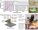
Motivating principles and setups for multispectral petrographic imaging with both reflected and
transmitted light. (A) The addition of bands within the sensitivity range of a standard optical sensor
allows for the sampling of distinctive spectral characteristics, such as the hematite peak and trough
near 750 nm and 850 nm, respectively. (B) Ultraviolet (UV) fluorescence is an informative source of
contrast when studying materials responsive to UV light, like the apatitic and organic components of
this fish fossil (from Tischlinger and Arratia, 2013). (C) Traditional cameras filter incoming light to
just red, green, and blue signals, limiting spectral range and reducing the spatial resolution of each
color. We use narrowband lights (one at a time), which allows us to capture signals from the full range
of sensitivity, and at the full resolution of the optical sensor. (D) Photograph of our setup.
RGB—red-green-blue; VNIR—visible to near-infrared.
Spectral Resolution
One of the key lessons learned from 50 years of satellite-based remote sensing of Earth’s surface is the
utility of bands outside the traditional red-green-blue (RGB) visible spectrum to take advantage of the
unique reflective characteristics of rocks and vegetation (Melesse et al., 2007). The reflective
properties of certain geological materials in the visible to near-infrared (VNIR; 300–1100 nm) spectrum
still apply at the scale of a hand sample and can be used by a petrographic camera to maximize feature
contrast and aid segmentation.
Increasing the range and number of light spectra imaged usually diminishes spatial resolution because
increasingly long wavelength (>1000 nm) and/or narrowband light sources are low intensity, meaning
cameras designed for hyperspectral imaging must have larger pixels to gather enough photons to form a
signal. Thus, we cannot design an imager with continuous spectral coverage throughout the VNIR spectrum
and instead choose to optimize for the trade-off between spatial and spectral resolution (Ma et al.,
2014). Our optical sensor (sensitive from 300 to 1000 nm) maintains the highest available spatial
resolutions while still detecting important spectral properties beyond RGB. In particular, metallic
oxides, clay minerals, pyroxenes, and olivines have absorption bands at wavelengths less than 1000 nm
that can enhance contrast between geological classes (Bishop et al., 2019; Fig. 1A).
We create color channels by illuminating samples with an array of eight Smart Vision S75 narrowband LEDs
(Fig. 1D), which can be chosen from any of the ten wavelengths shown in Figure 1A. We inform our
selection of lights through preliminary tests for maximized feature contrast and equip all lights with a
polarizing film to reduce glare.
Ultraviolet (UV) Fluorescence
In a dark laboratory setting, fluorescence from minerals like carbonates and phosphates can add contrast
when imaged in the visible spectrum. For example, in carbonate rocks at successive stages of calcite
precipitation, diagenesis, and recrystallization, differences in the trace element chemistry of the
stages will produce heterogeneities in the strength of fluorescence and thus contrast in the image
(Dravis and Yurewicz, 1985). Additionally, organic or apatitic fossil materials often fluoresce, making
UV fluorescence photography a valuable tool for creating contrast in paleontological samples
(Tischlinger and Arratia, 2013; Fig. 1B). To image fluorescence, we illuminate samples with a 365 nm
SmartVision LED. To reduce noise in the images, we place a bandpass filter with a cut-off wavelength of
395 nm over the UV light to remove any visible components of the emitted spectrum and use a 400 nm
cut-on UV filter in front of the lens to eliminate any UV light from reaching the camera sensor. Note
that when imaging with UV, the camera records the fluorescence of the materials in the VNIR spectrum.
Transmitted Light
Thin section transmitted light imagery offers another opportunity for increased contrast. Anisotropy,
cleavage, and twinning create distinctive qualities in grains and crystals within a thin section and
delineate grain boundaries (Rogers and Kerr, 1942). Additionally, crossed polarizers in transmitted
light setups heighten contrast between features by creating differential extinction and birefringence
patterns (Rogers and Kerr, 1942). To image thin sections with transmitted plane-polarized (PPL) and
cross-polarized (XPL) light, we have created a light table that can be used with GIRI or any camera
stand setup (Fig. 1D). The light source for this table is a dense Ramona Optics LED board with five
wavelengths (470, 530, 620, 850, 940 nm), which illuminates the sample through a diffuser and a
broadband linear polarizer. To image XPL, we attach a second polarizer over the sample, perpendicular to
the lower linear polarizer (Fig. 1D). Unlike traditional petrographic microscopes, this light table
holds the sample fixed, while a NEMA 17 stepper motor rotates both polarizers synchronously (Fueten,
1997) with a precision of 2.8 × 10⁻⁴ degrees.
Data Processing
In the case of both transmitted and reflected light, all captured image channels are perfectly aligned,
allowing the user to view any three channels in a false color image or analyze all captures as a single
multichannel image. Our setup, like all cameras, contends with chromatic aberration, whereby each
wavelength of light achieves maximal sharpness at a different focal depth due to the
wavelength-dependence of light refraction (Jacobson et al., 2013). In the supplemental
material1, we demonstrate how we apply blur modeling and deconvolution to achieve
multispectral images that are sharper than a standard RGB camera.
Results
In the following case studies, we illustrate two examples where the added spectral data from our
reflected and transmitted light setups enhance our ability to distinguish features within geological
samples. To classify pixels, we use a support vector machine (SVM), which is a simple machine learning
model, to show the potential for future machine learning efforts when trained on these more informative
spectral data.
Case Study 1: Feature Mapping in Reflected Light
A lack of contrast between classes in reflected light imagery commonly stems from all pixel values
falling near a brightness line—a 1:1 intensity line where values are well-correlated between channels
(Fig. 2B). In Figure 2A, we show an RGB image of an archaeocyathid boundstone sample, wherein each of
the four classes (dolomite, micritic calcite, archaeocyathid, and calcite-filled crack) shows
well-correlated pixel values (Fig. 2B). When segmenting these samples, the class overlap in RGB space
hinders pixel-wise classification, leading to uncertain boundaries between classes (Figs. 2D and 2E).
The same image in a UV-yellow-red colorspace (Fig. 2A) shows reduced channel covariance for all four
classes (Fig. 2C). With the new spectral information available in UV-yellow-red space, an SVM has 30%
improved accuracy, and produces resolved regions with distinct boundaries for each class (Figs. 2D and
2F).
 Figure
2
Figure
2
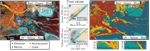
Improved segmentation results with multispectral reflected light imagery. (A) We take the same image of
an archaeocyathid boundstone sample in a traditional red-green-blue (RGB) colorspace, as well as a false
color ultraviolet (UV)-yellow-red space and sample the same pixels for four feature classes in each
(colored boxes). (B) In the RGB image, all classes show covariance between color channels, and most
pixels fall around the brightness line. (C) In the UV-yellow-red (UV-Y-R) image, covariance between
channels is removed for all classes, as evidenced by the fourfold increase in average distance between
each pixel and the brightness line (reported as total least squares, TLS). The movement of all classes
away from the brightness line into distinct regions of the color space eases segmentation. (D–F) Using a
support vector machine (SVM), an automated classification of the RGB image is 65% accurate and does not
give high-resolution borders between classes and regions (D, E). In contrast, an SVM segmentation of the
UV-yellow-red image is 91% accurate and gives sharp region and class boundaries more suitable for
measurements (D, F).
Case Study 2: Feature Mapping in Transmitted Light
A primary limitation of performing image analysis on thin sections with existing microscope cameras is
the FOV. In this example, we use a granite sample from the Golden Horn Batholith (Eddy et al., 2016)
that has crystals with diameters approaching 1 cm. Because these crystals are large relative to a
microscope FOV (Fig. 3A), the concentration of minerals in an image will be variable depending on the
portion of the thin section placed under the lens. For example, the concentration of plagioclase
assessed through classification may range from 29% to 55% when using the 2.5× objective on a
petrographic microscope (Fig. 3H). The variation in concentrations increases if magnification increases
(reducing FOV) or point counts are used to assess modality as opposed to pixel classifications (Fig.
3H).
 Figure
3
Figure
3
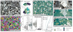
Improved modality data from multiple rotations of crossed polarizers for transmitted light imagery of
thin sections. (A) Red-green-blue (RGB), cross-polarized (XPL) image of a granite thin section from the
Golden Horn Batholith showing the full field of view (FOV) possible with our setup compared to those
obtainable with a microscope camera. (B) False color image obtained using green (530 nm) light at three
separate XPL orientations, 18° apart. (C) In principal component (PC) space, the pixel values for the
four mineral classes (quartz, plagioclase, orthoclase, and mafics) in a single rotation RGB XPL image
mostly overlap in one area of the plot. For an RGB XPL image containing five 18° rotations stacked into
a 15-channel image, the pixel values spread out into a cone, where the position on the cone occupied by
a given pixel relates to the class of the mineral and the relative orientation of its crystallographic
axis. This added separation of the classes in the PC space of the five rotation XPL image improves the
accuracy of pixel classifications from machine learning models, like the example given in (D). (E–G) In
a zoomed-in portion of the image (E), we see that a support vector machine (SVM) using just a single
rotation XPL RGB image (F) is 27% less accurate at classifying pixels compared to an SVM that is given
the five-rotation image (G). Even with accurate classifications, analyzing only a relatively small FOV
can add uncertainty. We see in (H) that the resulting modality data from the classification in (C) have
highly variable values when assessed within the FOV of a traditional petrographic microscope. Each point
in the plot represents the modality assessed in a randomly selected area of the segmentation equal to
the size of a microscope FOV using either a 2.5× or 10× objective. The variation in these errors between
classes stems from the characteristic size and relative abundance of the minerals. (I) To show the
effect of crystal size and abundance, we calculate the number of images that correctly estimate the
modality of a given mineral in a view size normalized to the mineral abundance (determined using a 4.5 ×
5.5 × 4 cm 3D grinding, imaging, and reconstruction instrument [GIRI] reconstruction of the sample). In
an experiment randomly drawing thin sections from the full volume of this granite sample, we see that an
approximately equal fraction of images estimates the mafic mineral modality within a 90% correctness
threshold when comparing GIRI to a 2.5× microscope objective. However, at the 95% threshold, as well as
with the larger plagioclase crystals, the GIRI FOV performs nearly twice as well.
This example also illustrates the benefit of building additional image channels from polarizer
orientations (as opposed to additional wavelengths of light). With a single RGB image from one
orientation of the crossed polarizers, capturing all possible birefringence and extinction properties
for a given mineral class in a training set can be difficult and time-consuming, and the end result can
be inaccurate classification (Fig. 3F). When multiple rotation XPL images are stacked together in the
training set, each pixel takes on a broader range of the color and textural properties that a mineral
may exhibit in cross-polarized light, which helps the machine learning model generalize and leads to
more accurate classifications with the same number of training samples (Figs. 3C, 3D, and 3G).
Discussion
Because our camera improves outcomes when using machine learning techniques to produce petrographic data,
we now are focused on high-throughput methods for complete sample image analyses within stratigraphic
sections or geologic maps. Our workflow takes the same samples gathered for geochemical or geophysical
laboratory analyses and photographs them as polished slabs and/or thin sections. As an example, we
created a bed-by-bed library containing nearly 2,000 images that chronicles paleoenvironmental change
through the lower Ordovician Kinblade Formation (Fig. 4). Within a single map or section, systematic
image analysis can yield lithofacies data that quantify spatio-temporal patterns in grain, crystal, and
fossil characteristics, while allowing new tests of geochemical interpretations (e.g., Geyman and
Maloof, 2021; Ahm et al., 2019).
 Figure
4
Figure
4
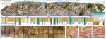
Example of a reproducible, quantitative lithofacies data set. (A) The lower Ordovician Kinblade
Formation outcropping in Ardmore Oklahoma (GPS location: 34.372821, –97.145353) is a 791 m succession of
carbonate strata containing 1,922 beds. (B) Following bed-by-bed field study, sampling, and geochemical
measurement, we epoxy 1 cm
2 chips from each sample for efficient grinding, polishing, and
imaging. The chip size is chosen to best encapsulate the dominant grain, fossil, and bedform sizes in
the data set. The resulting ~2,000 images (examples C–E, shown here in red-green-blue space, but all are
8-channel multispectral images) now are a documentation of the lithofacies in the measured section at
Ardmore and ready for image analysis, classification, segmentation, and interpretation.
At the same time, amassing a standardized, multispectral image library with annotated examples (Deng et
al., 2009) of geologic features from many localities will help train more general machine learning
models for petrography. These collections of slab and thin-section images are a first step toward the
goal of automated routines to measure features in rock samples from pictures. Curated image libraries
also can serve as a classroom tool for teaching petrography, and student work to classify images can
provide training examples for machine learning—a crowdsourcing technique that has seen recent success in
several fields (e.g., van den Bergh et al., 2021).
In addition to improving lithofacies data, we see our camera and petrographic images as a vehicle to
improve access and reproducibility in geology. Open access to archives like Integrated Ocean Drilling
Program (IODP) cores has expanded the number of people producing complementary data sets and provided
for deeper, more reproducible studies of Earth’s climate and oceans in recent geologic periods (Becker
et al., 2019). A similar framework should exist for rock outcrops that span deeper into Earth’s history,
where, currently, the observations that form geologic maps and stratigraphic sections tend to be
documented primarily in field notes or illustrative outcrop/sample photographs. For corroboration or
expansion upon previous outcrop-based studies, this system requires workers to visit the locality
themselves. Instead, open access to standardized petrographic image collections will allow broader
groups of researchers to measure and interpret features in rock formations from around the world,
enhancing both reproducibility (Baker, 2016) and diversity, equity, and inclusion (Fernandes et al.,
2020) in geology. Although our archives are not continuous records like IODP cores, they benefit from
the added spatial context available at rock outcrops and provide a zoomed-in perspective to supplement
constantly improving aerial survey techniques (Shah et al., 2021). In concert with satellite,
drone-derived, and hand-held imagery, our pipeline for systematic imaging, classification, and
measurement of rock samples can form an important layer in multiscale digitization and interpretation of
physical rock properties.
Acknowledgments
The authors would like to thank NSF EAR-1028768 and Princeton University for funding. Arnab Chatterjee
and Peter Siegel at Digital Transitions, Nolan Greve and Jeremy Brodersen at SmartVision Lights, Mark
Harfouche and Gregor Horstmeyer at Ramona Optics, and Dave Crawford and Jenifer Powell at Moxtek
provided support with the camera, lights, light table, and polarizers, respectively. We thank Bolton
Howes, Cedric Hagen, Brad Samuels, and Michael Eddy for useful discussions. We also appreciate the
constructive feedback received from reviewer Sarah Jacquet and editor James Schmitt.
References Cited
- Ahm, A.S.C., Bjerrum, C.J., Blättler, C.L., Swart, P.K., and Higgins, J.A., 2018, Quantifying early
marine diagenesis in shallow-water carbonate sediments: Geochimica et Cosmochimica Acta, v. 236, p.
140–159, https://doi.org/10.1016/j.gca.2018.02.042.
- Ahm, A.S.C., Maloof, A.C., Macdonald, F.A., Hoffman, P.F., Bjerrum, C.J., Bold, U., Rose, C.V.,
Strauss, J.V., and Higgins, J.A., 2019, An early diagenetic deglacial origin for basal Ediacaran
“cap dolostones”: Earth and Planetary Science Letters, v. 506, p. 292–307,
https://doi.org/10.1016/j.epsl.2018.10.046.
- Ahm, A.S.C., Bjerrum, C.J., Hoffman, P.F., Macdonald, F.A., Maloof, A.C., Rose, C.V., Strauss, J.V.,
and Higgins, J.A., 2021, The Ca and Mg isotope record of the Cryogenian Trezona carbon isotope
excursion: Earth and Planetary Science Letters, v. 568, 117002,
https://doi.org/10.1016/j.epsl.2021.117002.
- Baker, M., 2016, Reproducibility crisis: Nature, v. 533, p. 353–366.
- Becker, K., Austin, J.A., Exon, N., Humphris, S., Kastner, M., McKenzie, J.A., Miller, K.G.,
Suyehiro, K., and Taira, A., 2019, 50 Years of Scientific Ocean Drilling: Oceanography (Washington,
D.C.), v. 32, p. 17–21, https://doi.org/10.5670/oceanog.2019.110.
- Bergmann, K.D., Zentmyer, R.A., and Fischer, W.W., 2011, The stratigraphic expression of a large
negative carbon isotope excursion from the Ediacaran Johnnie Formation, Death Valley: Precambrian
Research, v. 188, p. 45–56, https://doi.org/10.1016/j.precamres.2011.03.014.
- Bishop, J.L., Bell, J.F., III, and Moersch, J.E., editors, 2019, Remote Compositional Analysis:
Techniques for Understanding Spectroscopy, Mineralogy, and Geochemistry of Planetary Surfaces.
Volume 24: Cambridge, UK, Cambridge University Press, https://doi.org/10.1017/9781316888872.
- Cesare, B., Campomenosi, N., and Shribak, M., 2022, Polychromatic polarization: Boosting the
capabilities of the good old petrographic microscope: Geology, v. 50, p. 137–141,
https://doi.org/10.1130/G49303.1.
- Corsetti, F.A., Kidder, D.L., and Marenco, P.J., 2006, Trends in oolite dolomitization across the
Neoproterozoic-Cambrian boundary: A case study from Death Valley, California: Sedimentary Geology,
v. 191, p. 135–150, https://doi.org/10.1016/j.sedgeo.2006.03.021.
- Dahl, T.W., Connelly, J.N., Li, D., Kouchinsky, A., Gill, B.C., Porter, S., Maloof, A.C., and
Bizzarro, M., 2019, Atmosphere-ocean oxygen and productivity dynamics during early animal
radiations: Proceedings of the National Academy of Sciences of the United States of America, v. 116,
p. 19,352–19,361, https://doi.org/10.1073/pnas.1901178116.
- Deng, J., Dong, W., Socher, R., Li, L.J., Li, K., and Fei-Fei, L., 2009, Imagenet: A large-scale
hierarchical image database: 2009 IEEE Conference on Computer Vision and Pattern Recognition: IEEE,
p. 248–255, https://10.1109/CVPR.2009.5206848.
- Dravis, J.J., and Yurewicz, D.A., 1985, Enhanced carbonate petrography using fluorescence
microscopy: Journal of Sedimentary Research, v. 55, p. 795–804.
- Dyer, B., Higgins, J.A., and Maloof, A.C., 2017, A probabilistic analysis of meteorically altered
δ13C chemostratigraphy from late Paleozoic ice age carbonate platforms: Geology, v. 45,
p. 135–138, https://doi.org/10.1130/G38513.1.
- Eddy, M.P., Bowring, S.A., Miller, R.B., and Tepper, J.H., 2016, Rapid assembly and crystallization
of a fossil large-volume silicic magma chamber: Geology, v. 44, p. 331–334,
https://doi.org/10.1130/G37631.1.
- Fernandes, A.M., Abeyta, A., Mahon, R.C., Martindale, R., Bergmann, K.D., Jackson, C., Present,
T.M., Swanson, T., Reano, D., Butler, K., Swanson, T., Butler, K., Brisson, S., Johnson, C., Mohrig,
D., and Blum, M.D., 2020, “Enriching Lives within Sedimentary Geology”: Actionable Recommendations
for Making SEPM a Diverse, Equitable and Inclusive Society for All Sedimentary Geologists:
EarthArXiv, https://doi.org/10.31223/osf.io/y7v9e.
- Fueten, F., 1997, A computer-controlled rotating polarizer stage for the petrographic microscope:
Computers & Geosciences, v. 23, p. 203–208, https://doi.org/10.1016/S0098-3004(97)85443-X.
- Geyman, E.C., and Maloof, A.C., 2021, Facies control on carbonate δ13C on the Great
Bahama Bank: Geology, v. 49, p. 1049–1054, https://doi.org/10.1130/G48862.1.
- Geyman, E.C., Maloof, A.C., and Dyer, B., 2021, How is sea level change encoded in carbonate
stratigraphy?: Earth and Planetary Science Letters, v. 560, 116790,
https://doi.org/10.1016/j.epsl.2021.116790.
- Halverson, G.P., Hoffman, P.F., Schrag, D.P., Maloof, A.C., and Rice, A.H.N., 2005, Toward a
Neoproterozoic composite carbon-isotope record: Geological Society of America Bulletin, v. 117, p.
1181–1207, https://doi.org/10.1130/B25630.1.
- Hay, C.C., Creveling, J.R., Hagen, C.J., Maloof, A.C., and Huybers, P., 2019, A library of early
Cambrian chemostratigraphic correlations from a reproducible algorithm: Geology, v. 47, p. 457–460,
https://doi.org/10.1130/G46019.1.
- He, K., Gkioxari, G., Dollár, P., and Girshick, R., 2017, Mask R-CNN: Proceedings of the 2017 IEEE
International Conference on Computer Vision, p. 2961–2969, https://10.1109/ICCV.2017.322.
- Higgins, M.D., 2000, Measurement of crystal size distributions: The American Mineralogist, v. 85, p.
1105–1116, https://doi.org/10.2138/am-2000-8-901.
- Hood, A.v., Planavsky, N.J., Wallace, M.W., Wang, X., Bellefroid, E.J., Gueguen, B., and Cole, D.B.,
2016, Integrated geochemical-petrographic insights from component-selective 238U of
Cryogenian marine carbonates: Geology, v. 44, p. 935–938, https://doi.org/10.1130/G38533.1.
- Jacobson, R., Ray, S., Attridge, G.G., and Axford, N., 2013, Manual of Photography: New York,
Routledge, 464 p., https://doi.org/10.4324/9780080510965.
- Koeshidayatullah, A., Morsilli, M., Lehrmann, D.J., Al-Ramadan, K., and Payne, J.L., 2020, Fully
automated carbonate petrography using deep convolutional neural networks: Marine and Petroleum
Geology, v. 122, 104687, https://doi.org/10.1016/j.marpetgeo.2020.104687.
- LeCun, Y., Boser, B., Denker, J., Henderson, D., Howard, R., Hubbard, W., and Jackel, L., 1989,
Handwritten digit recognition with a back-propagation network: Advances in Neural Information
Processing Systems, v. , p. 396–404.
- Li, X., Chen, H., Qi, X., Dou, Q., Fu, C.W., and Heng, P.A., 2018, H-DenseUNet: Hybrid densely
connected UNet for liver and tumor segmentation from CT volumes: IEEE Transactions on Medical
Imaging, v. 37, p. 2663–2674, https://doi.org/10.1109/TMI.2018.2845918.
- Lin, T.Y., Maire, M., Belongie, S., Hays, J., Perona, P., Ramanan, D., Dollár, P., and Zitnick,
C.L., 2014, Microsoft COCO: Common objects in context, in Fleet, D., Pajdla, T., Schiele,
B., and Tuytelaars, T., eds., Computer Vision—ECCV 2014: Lecture Notes in Computer Science: Berlin,
Springer, v. 8693, p. 740–755, https://doi.org/10.1007/978-3-319-10602-1_48.
- Ma, C., Cao, X., Tong, X., Dai, Q., and Lin, S., 2014, Acquisition of high spatial and spectral
resolution video with a hybrid camera system: International Journal of Computer Vision, v. 110, p.
141–155, https://doi.org/10.1007/s11263-013-0690-4.
- Maloof, A.C., Porter, S.M., Moore, J.L., Dudás, F.Ö., Bowring, S.A., Higgins, J.A., Fike, D.A., and
Eddy, M.P., 2010, The earliest Cambrian record of animals and ocean geochemical change: Geological
Society of America Bulletin, v. 122, p. 1731–1774, https://doi.org/10.1130/B30346.1.
- Mehra, A., and Maloof, A., 2018, Multiscale approach reveals that Cloudina aggregates are
detritus and not in situ reef constructions: Proceedings of the National Academy of Sciences, v. 15,
no. 11, https://doi.org/10.1073/pnas.1719911115.
- Melesse, A.M., Weng, Q., Thenkabail, P.S., and Senay, G.B., 2007, Remote sensing sensors and
applications in environmental resources mapping and modelling: Sensors (Basel), v. 7, p. 3209–3241,
https://doi.org/10.3390/s7123209.
- Neilson, M., and Brockman, G., 1977, The error associated with point-counting: The American
Mineralogist, v. 62, p. 1238–1244.
- Rogers, A.F., and Kerr, P.F., 1942, Optical Mineralogy: New York, McGraw-Hill.
- Shah, A.K., Morrow, R., Pace, M., Harris, M.S., and Doar, W., III, 2021, Mapping critical minerals
from the sky: GSA Today, v. 31, https://doi.org/10.1130/GSATG512A.1.
- Shand, S., 1916, A recording micrometer for geometrical rock analysis: The Journal of Geology, v.
24, p. 394–404, https://doi.org/10.1086/622346.
- Solomon, M., 1963, Counting and sampling errors in modal analysis by point counter: Journal of
Petrology, v. 4, p. 367–382, https://doi.org/10.1093/petrology/4.3.367.
- Soomro, T.A., Khan, M.A., Gao, J., Khan, T.M., and Paul, M., 2017, Contrast normalization steps for
increased sensitivity of a retinal image segmentation method: Signal, Image and Video Processing, v.
11, p. 1509–1517, https://doi.org/10.1007/s11760-017-1114-7.
- Tian, Y., Pei, K., Jana, S., and Ray, B., 2018, Deeptest: Automated testing of
deep-neural-network-driven autonomous cars: Proceedings of the 40th International Conference on
Software Engineering, p. 303–314, https://doi.org/10.1145/3180155.3180220.
- Tischlinger, H., and Arratia, G., 2013, Ultraviolet light as a tool for investigating Mesozoic
fishes, with a focus on the ichthyofauna of the Solnhofen archipelago, in Arratia, G.,
Schultze, H.-P., and Wilson, M.V.H., eds., Mesozoic Fishes 5—Global Diversity and Evolution:
München, Germany, Verlag Dr. Friedrich Pfeil, p. 549–560.
- van den Bergh, J., Chirayath, V., Li, A., Torres-Perez, J.L., and Segal-Rozenhaimer, M., 2021,
NeMO-Net—Gamifying 3D labeling of multi-modal reference datasets to support automated marine habitat
mapping: Frontiers in Marine Science, v. 8, p. 347, https://doi.org/10.3389/fmars.2021.645408.
- Yesiloglu-Gultekin, N., Keceli, A.S., Sezer, E.A., Can, A.B., Gokceoglu, C., and Bayhan, H., 2012, A
computer program (TSecSoft) to determine mineral percentages using photographs obtained from thin
sections: Computers & Geosciences, v. 46, p. 310–316,
https://doi.org/10.1016/j.cageo.2012.01.001.