Introduction and Background
Rapid improvements in the fidelity of consumer-grade cameras, coupled with novel computer vision–based
photogrammetric image processing pipelines (i.e., structure from motion–multiview stereo photogrammetry:
SfM-MVS), have revolutionized outcrop studies over the past decade, bringing traditional field geology
into the digital age. These developments are also closely tied to major methodological improvements for
virtual outcrop model (VOM) interpretation. All these advancements have accelerated the use of digital
outcrop data capture and analysis in field geology, transforming what was principally a visualization
medium into fully interrogatable quantitative geo-data objects (Jones et al., 2004; Bemis et al., 2014;
Howell et al., 2014; Hodgetts et al., 2015; Biber et al., 2018; Bruna et al., 2019; Caravaca et al.,
2019; Thiele et al., 2019; Triantafyllou et al., 2019). Initially, close-range remote-sensing studies
seeking to reconstruct and analyze rock outcrops were dominantly built around terrestrial laser scanning
systems (terrestrial lidar), which became commercially available around two decades ago (e.g., Bellian
et al., 2002). These initial works tended to be technology demonstrations rather than routine field
studies, with the expense, weight, and challenging operational learning curve limiting replication to a
few highly specialized geospatial specialists and groups. Receiving greater interest from the
archaeological community, the adoption of digital photogrammetry by outcrop geologists was initially
slow (e.g., Hodgetts et al., 2004; Pringle et al., 2004), with legacy photogrammetric reconstruction
techniques requiring highly specialized, expensive metric cameras or software (Chandler and Fryer,
2005), and commonly carried the limitation of cumbersome manual assignment of key points on the targeted
rock surface (e.g., Simpson et al., 2004). Many of these disadvantages were addressed with the advent of
low-cost or open-source SfM-MVS photogrammetry image processing pipelines (e.g., Snavely et al., 2006;
Furukawa and Ponce, 2009; Wu, 2011), which facilitated the use of uncalibrated consumer-grade cameras
and enabled automated image key-point detection and matching (e.g., James and Robson, 2012). The
potential of producing 3D rock-surface models using consumer-grade cameras attracted the interest of
numerous workers. These developments coupled with the increasing availability of lightweight and
low-cost drones able to carry cameras and other sensors, have finally boosted the use of SfM-MVS
reconstruction in geosciences.
For many geoscience applications, it is necessary to register 3D rock-surface reconstructions within a
local or global coordinate frame. The use of survey-grade total stations and/or real-time kinematic
(RTK) differential global navigation satellite system (GNSS) antennas permit both terrestrial (Jaud et
al., 2020) and aerial (Rieke et al., 2012) image data and/or ground control points (GCPs) to be
georeferenced within the mapped scene with centimeter to millimeter accuracy (Bemis et al., 2014). Those
survey tools are, however, bulky and expensive, and are not standard tools for geoscientists engaged in
fieldwork. Improvements in consumer-grade GNSS receivers, capable of harnessing multiple constellations
(i.e., GPS, Glonass, Galileo, and BeiDou), now permit model geo-registration with greater simplicity and
accuracies that are acceptable for many geoscientific applications. Most current smartphones are
equipped with such GNSS chipsets, which enable the positioning of photos and GCPs with meter-level
accuracy, or even spatial-decimeter accuracy for dual-frequency chipsets, with >20 min acquisition
times for individual locations (Dabove et al., 2020; Uradziński and Bakuła, 2020). Under these
conditions, the use of smartphones permits georeferencing of >~100-m-wide photogrammetric models
generated via terrestrial imagery (Fig. 1). The availability of photo orientation information, provided
by the smartphone’s inertial measurement unit (especially the magnetometer and gyroscope/accelerometer
sensors), in conjunction with the GNSS position, can further improve the quality of the model
registration procedure. Indeed, the photo orientation information mitigates the positional error
associated with the Z component, and full georeferencing of >50–60-m-wide exposures can be achieved
with a consumer-grade dual-frequency GNSS chipset–equipped smartphone (Tavani et al., 2019, 2020).
 Figure
1
Figure
1
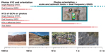
Scale-ranges of applicability of different methods for the registration of 3D models of outcrops, and
tools used in this work. GCPs—ground control points; GNSS—global navigation satellite system;
RTK—real-time kinematic.
Confident georeferencing of smaller-scale outcrops with minimal equipment, however, remains challenging,
limiting the utility of photogrammetric acquisition in routine geological fieldwork. In this article, we
present a workflow using a smartphone and minimal accessories to address this challenge (Fig. 1) and
demonstrate the applicability of using smartphone photo and video surveys of an active fault in the
Apennines (Italy). Those 3D models are georeferenced by integrating the use of Agisoft Metashape and
OpenPlot software tools (Tavani et al., 2019).
Methods and Data
The Acquisition Site
The survey method proposed herein was performed on an outcrop of an active normal fault located within
the Apennines, central Italy. A high-resolution 3D surface reconstruction of the outcrop is already
available (Corradetti et al., 2021), thus allowing us to compare our results with a ground-truth model.
The area contains outcropping Mesozoic rocks affected by active normal faulting. For the aforementioned
survey, we focused upon one segment striking N135°–160° (Fig. 2A). A wide (~0.3–1 m) portion of this
fault was exposed after the dramatic MW 6.5 earthquake that struck the area on 30 Oct. 2016 (e.g.,
Chiaraluce et al., 2017), offering the opportunity to study this “fresh” portion of the fault surface
(the white ribbon shown over the bottom of the fault surface in Fig. 2A).
 Figure
2
Figure
2
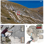
Photograph of the active normal fault modeled in this work (A). (B) Field set up and measurements taken
before image acquisition. A ruler is used to measure the length between two points, each photographed
for later recognition. A stand (compass holder, CH) is placed on the outcrop and its attitude measured
defining the CH strike. The operator can then proceed with the photo/video acquisition providing that
the CH is left on the outcrop to be included in the model. (C) Dense point cloud of the Photo Model. In
the model, four markers are added, representing the two points whose distance was measured with the
tape, and two points along the CH strike. The θ, ξ, and ρ vectors of the images are also indicated.
Pre-Acquisition Setup
Image acquisition was carried out on 30 Oct. 2020, between 12:46 p.m. and 1:01 p.m., using a
dual-frequency GNSS-equipped smartphone (Xiaomi 9T pro), hand-held gimbal, compass holder,
compass-clinometer, and metric tape measure (see Fig. 1). In the field (Fig. 2B), the compass holder was
placed within the scene using a detachable sticky pad with its edge approximately horizontal in relation
to the Earth frame, and its trend (CH strike in Fig. 2C) measured using a Brunton TruArc 20 compass. The
metric tape was used to measure the distance between two arbitrary features that later must be
identified in the 3D model to provide its scaling factor. Both the compass and the metric measuring tape
were removed before scene acquisition.
Image Acquisition
We produced two digital models of the fault using different approaches. The first model (from here on
referred to as the Photo Model) was generated using 200 photos (4000 × 2250 pixels and 4.77 mm focal
length). The second model (from here on referred to as the Video Model) was built using 528 photos (3840
× 2160 pixels and 4.77 mm focal length) extracted using VLC software from a 257-second-long video file
(i.e., 2.6 frames per second). Both acquisitions were carried out using the smartphone mounted on a DJI
OM4 gimbal, at a distance of ~30 cm from the fault plane. To include images oblique to the fault plane,
required to mitigate doming of the reconstructed scene (James and Robson, 2014; Tavani et al., 2019),
the view direction was repeatedly changed within an ~60° wide cone. Nevertheless, avoiding
operator-induced shadows into the scene meant that the main acquisition was sub-perpendicular to the
strike of the fault, being ~ENE.
Image Processing and Model Registration
Images were processed in Agisoft Metashape (version 1.6.2), resulting in two unregistered dense point
clouds (Fig. 2C). Four specific markers were manually added in Metashape. In Figure 2C, Point 1 and
Point 2 represent the two points whose distance was manually measured in the field. Point 3 and Point 4
were instead picked along one edge of the digitized compass holder (CH; Fig. 2C). These are used to
retrieve the trend of the CH strike, here coinciding with the strike of the fault plane. The rotational
transformation is the most critical aspect of model registration for many geoscience applications (e.g.,
discontinuity, bedding plane, or geobody orientation analysis). Our survey carries different assumptions
for the orientation of photographs: the short axis of the photo (θ in Fig. 2C) is pointing upward; the
view direction (ξ in Fig. 2C) is gently plunging and at a high angle to the fault plane; the long axis
of the photo (ρ in Fig. 2C) is lying horizontal, due to gimbal stabilization. The goal is to use the
stabilized direction of the long axis of photos to register the vertical axis and the markers placed on
the CH (defining the CH strike) to reorient the model around this vertical axis. This is done after
exporting from Metashape the cameras’ extrinsic parameters using the N-View Match (*.nvm) file format.
The exported data include θ, ξ, and ρ vectors expressed in the arbitrary reference frame. Then, we
exported the markers in *.txt format, which saves the estimated position of markers in the arbitrary
reference frame. These files are imported in OpenPlot, where the photos’ directions and the CH strike
are computed and graphed in a stereoplot (Plot 1 in Fig. 3). For both Photo and Video models, the ρ
direction is clustered along a great circle, which, thanks to the gimbal, represents the horizontal
plane in the real-world frame. For each model, the entire data set (i.e., the three directions of photos
and the four markers) are rotated to set the ρ great circle horizontal (Plot 2 in Fig. 3). Notice that
the rotation axis is univocally defined, being coincident to the strike of the best-fit plane. The
amount of rotation instead can be either the dip of the plane or 180° + dip. The correct placement of
the view direction (ξ) means that the selection between these two options by the user is trivial. The
resulting trend of the CH strike is N211° and N105° for the Photo and Video models, respectively. A
rotation about the vertical axis (57° counterclockwise for the Photo Model and 49° clockwise for the
Video Model) was applied to the entire data set to match the CH strike to its measured value, i.e.,
N154° (Plot 3 in Fig. 3). The twice- rotated markers were then scaled using the measured distance
between Point 1 and Point 2 and were eventually fully georeferenced using the measured position of Point
1. These two steps are achieved during the export stage from OpenPlot, which compiles a *.txt file
containing the correctly georeferenced coordinates of the four markers. This file was imported into
Metashape, which allows the direct georeferencing of the model. The whole procedure, from the export or
unregistered data from Metashape, through the rotations, scaling, and referencing in OpenPlot and the
final re-import in Metashape takes just a few minutes and can be followed step-by-step in the
supplementary video provided (see Supplementary Material1). A good practice consists of
checking the results and re-exporting the cameras’ extrinsic data of the registered model to possibly
repeat the procedure if residual rotations occur (i.e., if ρ is not perfectly lying on a horizontal
plane), which may relate to the proximity of the markers used for the transform and on their positional
accuracy.
 Figure
3
Figure
3
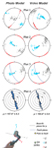
Lower hemisphere stereographic projection (stereonet) of the camera vectors for both the Photo and Video
models, after model building (Plot 1), and after horizontalization of the ρ-vector great-circle envelope
(Plot 2). In essence, after this rotation, the vertical axis is paralleled to the true vertical, but the
azimuth is yet randomly oriented. (Plot 3) Stereonet of the camera vectors after rotation around the
vertical axis. (Plot 4) Rose diagram showing the distribution of the ρ vectors in both models.
CH—compass holder.
Results
For the Photo Model, all of the 200 uploaded photos were successfully aligned and used to produce a point
cloud made of ~6 × 10⁷ points (Fig. 4A). For the Video Model, we uploaded 735 video frames,
but only 528 of them were successfully aligned and used to produce a dense cloud of ~11.6 ×
107 points (Fig. 4A). Some of the excluded images were manually removed after alignment,
improving the quality of the 3D scene reconstruction. These images were identified through manual
selection of points associated with unrealistic or blurry geometries within the sparse cloud. Often
those were frames characterized by extreme overlap.
Both point clouds are characterized by zones on their boundaries, in which the 3D scene reconstruction
relies on oblique images (Fig. 4B). These zones are asymmetrical, due to the aforementioned obliquity
between the fault-perpendicular direction and the average photo view direction. Accordingly, we cropped
the point clouds to exclude these zones and areas where the 3D reconstruction relied upon less than nine
images (Fig. 4B).
 Figure
4
Figure
4
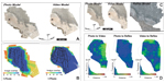
The Photo and Video models dense point cloud (A). (B) Images positions with respect to the models and
number of images overlapping areas. (C) Cropped Photo and Video models. The Reflex Model from Corradetti
et al. (2021). (D) Cloud to cloud distance between each pair of point clouds computed in CloudCompare.
The cropped point cloud for the Photo Model is composed of ~2.5 × 10⁷ points, whereas the
cropped Video Model consists of ~7.8 × 10⁷ points (Fig. 4C). The accuracy of these 3D surface
reconstructions was tested by generating difference maps from the two smartphone-generated models, and
between each smartphone-generated model and a high-resolution ground-truth model (from here on referred
to as the Reflex Model) built in 2016 using an image survey captured from the same outcrop with a dSLR
camera (Fig. 4C). In this regard, the same fault was mapped in 2016 (Corradetti et al., 2021), using 640
images (4272 × 2848 pixels) taken with a Canon EOS 450D reflex mounted on a tripod to suppress motion
blur. The reconstructed area for the Reflex Model was ~2.67 m2, and the point cloud included
~2.7 × 10⁸ points. These three point clouds were uploaded in CloudCompare (Girardeau-Montaut,
2015), where they were first manually aligned using ~15 control points for each matched point cloud, and
then they were compared using the cloud-to-cloud distance tool. The resulting distance among the three
clouds was generally below 4 mm (Fig. 4D), which decreases down to <2 mm for the Photo Model versus
Reflex Model.
The georeferenced Photo and Video models were then compared to evaluate differences in scaling and
rotation (translation was not investigated here). To achieve this, we uploaded the two scaled and
rotated models, using the compass holder as the origin of the reference frame. We aligned the two clouds
using 15 control points, and the result is a transformation matrix indicating that to align the two
point clouds, a scaling factor of 1.0012 is required. The rotations around the X, Y, and Z axes are
–0.38°, 1.00°, and 0.34° (1.1° around the strike direction and 0.29° around the horizontal direction
perpendicular to the strike).
Discussion
We have described a workflow for generating georeferenced 3D models of geological outcrops ranging in
size from tens of meters down to a few centimeters. The required tools are extremely portable. Their use
in the field is straightforward, with survey acquisition taking a few minutes for our case study. During
the development and testing of the procedure, it was notable that video sequence acquisition can provide
a more coherent scene, assuming that the mapped area is relatively continuous. On the other hand, video
sequences may generate excessive scene overlap, complicating image matching. Also, the use of video
frames implies the lack of control on shutter speed, aperture, ISO, etc., limiting the use of video
frames mostly to small outcrops. Thus, selectively captured still images generally ensure a better
result and a shorter processing time, as long as the acquisition is correctly carried out. Video models
instead provide a simpler acquisition scheme, albeit with greater risk of reconstruction artifacts.
Once the models are built, post-processing registration using the proposed method is also straightforward
for geoscientists with limited knowledge of geospatial data processing and analysis. From a practical
point of view, the use of a low-cost, lightweight gimbal smartphone stabilizer offers a key improvement
to similar workflows proposed previously (e.g., Tavani et al., 2020), and it is encouraged that
geoscientists who want to replicate the presented acquisition strategy include this item as part of
their standard equipment. Using a gimbal offers two substantial advantages. First, stabilization of the
smartphone during acquisition improves image quality (i.e., by limiting motion blur), with the produced
3D model rivaling an equivalent surface reconstruction produced with a higher resolution dSLR mounted on
a tripod. The second but most fundamental advantage of using a gimbal is the stabilization of the
smartphone along its long axis, so that all the images produced are oriented along a horizontal plane,
providing a constraint for our georeferencing procedure.
Two data sets, (i.e., photos and images extracted from a video sequence) have been tested to produce and
later register the Photo and Video models, respectively. These models have been compared together and
with the Reflex Model, which represents a benchmark build with photos obtained in 2016, although
probably minor morphological changes due to weathering can have occurred since then. Manual alignment of
the Photo and Video models shows that discrepancies ranging from 0 to 5 mm occur between the surface
reconstructions. There are notable discrepancies between the Video and Reflex models, whereas the Photo
and Reflex models are much more comparable, with surface displacements ranging between 0 and 2 mm.
Despite the lower number of input photos, the Photo Model outperforms the Video Model in terms of
accuracy. The major reason for this is the problematic reconstruction of the scene from extremely narrow
baseline images extracted from the video sequence. Despite the video capture having a more
straightforward acquisition procedure, it may require a more complex and time-consuming user-assisted
procedure of image selection and repeated runs of photo alignment.
Apart from minor differences in reconstruction quality and errors that may arise from manual detection of
the key points used in the similarity transform, the registration procedure of the two
smartphone-generated models led to models with consistent orientation and scaling characteristics. In
detail, we observed a rotation about the vertical axis of 0.34°. This error, which mostly relates to
digitization of the reconstructed CH placed within the scene, is negligible for many geological
applications, particularly if compared with the accuracy of analog compasses (e.g., Allmendinger et al.,
2017). Such minimal value, however, does not reflect field measurement accuracy, since only one
measurement was made of the same object present in the two models. Models of the same geological object,
created by different individuals at different times, could introduce additional rotational errors. A
slight misalignment of the registered horizon between the two models is reflected by the observed
rotations around the x and y axes of –0.38° and 1.00°, respectively. This misalignment
is attributable to the procedure of horizontalization of ρ: as seen in the rose diagram of Figure 3, ρ
in both models is clustered along a direction that is nearly parallel to the strike of the fault,
providing a greater constraint along the fault parallel direction than along its perpendicular. Indeed,
the discrepancy in the estimated horizontal plane between the two models, considering the orientation of
the fault, is 1.1° around the strike direction and 0.29° around the horizontal direction perpendicular
to the fault’s strike. In other words, the registration of the horizontal plane is sensitive to the
orientation of the photographs, so that the inclusion of oblique to the scene photographs may improve
the “horizontalization” of ρ.
Conclusion
This paper faces the need encountered by many field geologists to efficiently capture images of outcrops
with ultra-portable tools to produce detailed, scaled, and properly oriented “pocket” 3D digital
representations of rock exposures. Submillimeter point-cloud resolution is achieved with the suggested
procedure, equaling that of models obtained by means of reflex cameras, and proving the efficiency of
the proposed registration procedure for several quantitative applications in geology (e.g., fracture and
fault orientation and associated kinematic indicators, bedding attitude and thickness, fault roughness,
etc.). Furthermore, the proposed method is intuitive so that it can be applied by all geoscientists
irrespective of background or experience. In this regard, we hope that this workflow will favor the
widespread use of 3D models from smartphones.
References Cited
- Allmendinger, R.W., Siron, C.R., and Scott, C.P., 2017, Structural data collection with mobile
devices: Accuracy, redundancy, and best practices: Journal of Structural Geology, v. 102, p. 98–112,
https://doi.org/10.1016/j.jsg.2017.07.011.
- Bellian, J.A., Jennette, D.C., Kerans, C., Gibeaut, J., Andrews, J., Yssldyk, B., and Larue, D.,
2002, 3-dimensional digital outcrop data collection and analysis using eye-safe laser (LIDAR)
technology: American Association of Petroleum Geologists Search and Discovery Article 40056,
https://www.searchanddiscovery.com/documents/beg3d/ (last accessed 27 Feb. 2021).
- Bemis, S.P., Micklethwaite, S., Turner, D., James, M.R., Akciz, S., Thiele, S.T., and Bangash, H.A.,
2014, Ground-based and UAV-based photogrammetry: A multi-scale, high-resolution mapping tool for
structural geology and paleoseismology: Journal of Structural Geology, v. 69, p. 163–178,
https://doi.org/10.1016/j.jsg.2014.10.007.
- Biber, K., Khan, S.D., Seers, T.D., Sarmiento, S., and Lakshmikantha, M.R., 2018, Quantitative
characterization of a naturally fractured reservoir analog using a hybrid lidar-gigapixel imaging
approach: Geosphere, v. 14, p. 710–730, https://doi.org/10.1130/GES01449.1.
- Bruna, P.O., Straubhaar, J., Prabhakaran, R., Bertotti, G., Bisdom, K., Mariethoz, G., and Meda, M.,
2019, A new methodology to train fracture network simulation using multiple-point statistics: Solid
Earth, v. 10, p. 537–559, https://doi.org/10.5194/se-10-537-2019.
- Caravaca, G., Le Mouélic, S., Mangold, N., L’Haridon, J., Le Deit, L., and Massé, M., 2019, 3D
digital outcrop model reconstruction of the Kimberley outcrop (Gale crater, Mars) and its
integration into virtual reality for simulated geological analysis: Planetary and Space Science, v.
182, 104808, https://doi.org/10.1016/j.pss.2019.104808.
- Chandler, J.H., and Fryer, J.G., 2005, Recording aboriginal rock art using cheap digital cameras and
digital photogrammetry, in Proceedings of CIPA (Comité International de la Photogrammétrie
Architecturale [International Committee of Architectural Photogrammetry], p. 193–198,
https://www.cipaheritagedocumentation.org/wp-content/uploads/2018/12/Chandler-Fryer-Recording-aboriginal-rock-art-using-cheap-digital-cameras-and-digital-photogrammetry.pdf
(last accessed 6 June 2021).
- Chiaraluce, L., et al., 2017, The 2016 central Italy seismic sequence: A first look at the
mainshocks, aftershocks, and source models: Seismological Research Letters, v. 88, p. 757–771,
https://doi.org/10.1785/0220160221.
- Corradetti, A., Zambrano, M., Tavani, S., Tondi, E., and Seers, T.D., 2021, The impact of weathering
upon the roughness characteristics of a splay of the active fault system responsible for the massive
2016 seismic sequence of the Central Apennines, Italy: Geological Society of America Bulletin, v.
133, p. 885–896, https://doi.org/10.1130/B35661.1.
- Dabove, P., Di Pietra, V., and Piras, M., 2020, GNSS positioning using mobile devices with the
android operating system: ISPRS International Journal of Geo-Information, v. 9,
https://doi.org/10.3390/ijgi9040220.
- Furukawa, Y., and Ponce, J., 2009, Accurate, dense, and robust multiview stereopsis: IEEE
Transactions on Pattern Analysis and Machine Intelligence, v. 32, p. 1362–1376,
https://doi.org/10.1109/TPAMI.2009.161.
- Girardeau-Montaut, D., 2015, Cloud compare—3D point cloud and mesh processing software: Open Source
Project, https://www.danielgm.net/cc/ (last accessed 6 June 2021).
- Hodgetts, D., Drinkwater, N.J., Hodgson, J., Kavanagh, J., Flint, S.S., Keogh, K.J., and Howell,
J.A., 2004, Three-dimensional geological models from outcrop data using digital data collection
techniques: An example from the Tanqua Karoo depocentre, South Africa, in Curtis, A., and
Wood., R., eds., Geological Prior Information: Informing Science and Engineering: Geological
Society, London, Special Publication 239, p. 57–75, https://doi.org/10.1144/GSL.SP.2004.239.01.05.
- Hodgetts, D., Seers, T., Head, W., and Burnham, B.S., 2015, High performance visualisation of
multiscale geological outcrop data in single software environment, in 77th EAGE Conference
and Exhibition 2015: European Association of Geoscientists & Engineers, p. 1–5,
https://doi.org/10.3997/2214-4609.201412862.
- Howell, J.A., Martinius, A.W., and Good, T.R., 2014, The application of outcrop analogues in
geological modelling: A review, present status and future outlook, in Martinius, A.W.,
Howell, J.A., and Good, T.R., eds., Sediment-Body Geometry and Heterogeneity: Analogue Studies for
Modelling the Subsurface: Geological Society, London, Special Publication 387, p. 1–25,
https://doi.org/10.1144/SP387.12.
- James, M.R., and Robson, S., 2012, Straightforward reconstruction of 3D surfaces and topography with
a camera: Accuracy and geoscience application: Journal of Geophysical Research, v. 117, F03017,
https://doi.org/10.1029/2011JF002289.
- James, M.R., and Robson, S., 2014, Mitigating systematic error in topographic models derived from
UAV and ground-based image networks: Earth Surface Processes and Landforms, v. 39, p. 1413–1420,
https://doi.org/10.1002/esp.3609.
- Jaud, M., Bertin, S., Beauverger, M., Augereau, E., and Delacourt, C., 2020, RTK GNSS-assisted
terrestrial SfM photogrammetry without GCP: Application to coastal morphodynamics monitoring: Remote
Sensing, v. 12, p. 1889, https://doi.org/10.3390/rs12111889.
- Jones, R.R., McCaffrey, K.J.W., Wilson, R.W., and Holdsworth, R.E., 2004, Digital field data
acquisition: Towards increased quantification of uncertainty during geological mapping, in
Curtis, A., and Wood., R., eds., Geological Prior Information: Informing Science and Engineering:
Geological Society, London, Special Publication 239, p. 43–56,
https://doi.org/10.1144/GSL.SP.2004.239.01.04.
- Pringle, J.K., Westerman, A.R., Clark, J.D., Drinkwater, N.J., and Gardiner, A.R., 2004, 3D
high-resolution digital models of outcrop analogue study sites to constrain reservoir model
uncertainty: An example from Alport Castles, Derbyshire, UK: Petroleum Geoscience, v. 10, p.
343–352, https://doi.org/10.1144/1354-079303-617.
- Rieke, M., Foerster, T., Geipel, J., and Prinz, T., 2012, High-precision positioning and real-time
data processing of UAV-systems: ISPRS International Archives of the Photogrammetry: Remote Sensing
and Spatial Information Sciences, v. XXXVIII-1, C22, p. 119–124,
https://doi.org/10.5194/isprsarchives-XXXVIII-1-C22-119-2011.
- Simpson, A., Clogg, P., Díaz-Andreu, M., and Larkman, B., 2004, Towards three-dimensional
non-invasive recording of incised rock art: Antiquity, v. 78, p. 692–698,
https://doi.org/10.1017/S0003598X00113328.
- Snavely, N., Seitz, S.M., and Szeliski, R., 2006, Photo tourism: ACM Transactions on Graphics, v.
25, p. 835, https://doi.org/10.1145/1141911.1141964.
- Tavani, S., Corradetti, A., Granado, P., Snidero, M., Seers, T.D., and Mazzoli, S., 2019,
Smartphone: An alternative to ground control points for orienting virtual outcrop models and
assessing their quality: Geosphere, v. 15, p. 2043–2052, https://doi.org/10.1130/GES02167.1.
- Tavani, S., Pignalosa, A., Corradetti, A., Mercuri, M., Smeraglia, L., Riccardi, U., Seers, T.,
Pavlis, T., and Billi, A., 2020, Photogrammetric 3D model via smartphone GNSS sensor: Workflow,
error estimate, and best practices: Remote Sensing, v. 12, 3616, https://doi.org/10.3390/rs12213616.
- Thiele, S.T., Grose, L., Cui, T., and Cruden, A.R., 2019, Extraction of high-resolution structural
orientations from digital data: A Bayesian approach: Journal of Structural Geology,
https://doi.org/10.1016/j.jsg.2019.03.001.
- Triantafyllou, A., Watlet, A., Le Mouélic, S., Camelbeeck, T., Civet, F., Kaufmann, O., Quinif, Y.,
and Vandycke, S., 2019, 3-D digital outcrop model for analysis of brittle deformation and
lithological mapping (Lorette cave, Belgium): Journal of Structural Geology, v. 120, p. 55–66,
https://doi.org/10.1016/j.jsg.2019.01.001.
- Uradziński, M., and Bakuła, M., 2020, Assessment of static positioning accuracy using low-cost
smartphone GPS devices for geodetic survey points’ determination and monitoring: Applied Sciences
(Switzerland), v. 10, p. 1–22, https://doi.org/10.3390/app10155308.
- Wu, C., 2011, VisualSFM: A visual structure from motion system: http://ccwu.me/vsfm/ (last accessed
6 June 2021).