Introduction
The granite outcrop in Figure 1A is clearly deformed, with a nice shear fabric running from lower left to
upper right in the photo, and a field geologist could easily measure its orientation with a compass. How
strong is the fabric? That is harder to quantify, and the geologist would likely apply an adjective such
as “moderate” or “strong” in the field and bring an oriented sample back to the lab for further analysis
if desired.
 Figure
1
Figure
1
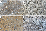
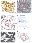
Examples of difficult field problems that can be solved with StraboTools. Answers are in Appendix 1. (A)
Deformed granite. The foliation is obvious and easy to measure, but quantifying its strength is
difficult to do in the field. (B) Subtly deformed image of a granodiorite outcrop. Do you see a fabric?
What deformation was applied? (C) Shadowed outcrop photograph of a cliff in alluvial fan deposits. Is
there a pebble imbrication indicating the direction of stream flow? (D) What is the proportion of dark
minerals in this granodiorite?
Is the granodiorite in Figure 1B deformed? Most observers would say no, but this image, of an originally
isotropic granodiorite, was digitally distorted by flattening in one direction and stretching in the
perpendicular direction (pure shear). We venture that few would call this a measurable fabric in the
field. Being able to detect and measure such subtle features would greatly aid studies of deformation,
flow alignment, and related fabrics.
Is there a pebble imbrication in Figure 1C that gives the local direction of current flow? What is the
proportion of dark minerals in Figure 1D? These can be difficult questions to answer, and recently at
the outcrop in Figure 1D, several professional geologists gave answers ranging from 5% to 30%. This
illustrates how difficult this simple and important measurement can be using the eye alone.
This sort of observation and measurement has occupied much of the field workflow in structural geology,
petrology, and sedimentary geology for a century or more. Still, such work can be frustratingly
qualitative and incomplete. Quantitative and repeatable measurements are the backbone of much of
scientific inquiry, yet field geologists have few tools available for making them on many types of
features.
Today, tools available to the field geologist are much the same as they were a century ago: devices for
measuring angles, bearings, and distances, and a few categorical measurement aids such as an acid bottle
and a magnet. Although mobile phones and laser rangefinders are replacing the compasses and tape
measures of yore, the domain of properties that can be measured is largely the same. Field studies are
typically the prelude to a comprehensive set of laboratory measurements of chemical composition,
porosity, mineral age, mineral or clast preferred orientation, remanent magnetism, and other useful
things. Such laboratory studies could be significantly enhanced if some of these properties could be
measured in the field. If such measurements could become routine and ubiquitous, then field studies
would produce richer results.
It is possible to bring devices into the field to measure chemical composition, magnetic susceptibility,
gamma-ray emissions, rock hardness, and other rock properties. These tools are valuable for mapping
subtle variations that may be unmappable by eye (e.g., Parkinson, 1996; Aydin et al., 2007; Dühnforth et
al., 2010; Coleman et al., 2012), but they are expensive and not widely employed. As a result, aside
from orientation measurements, fieldwork is still done in a mostly qualitative or semiquantitative
manner, using phrases such as “strong fabric,” “coarse-grained,” “dark,” or “poorly sorted,” rather than
quantitative measures. For structural analysis, several algorithms have been developed for
semi-automated fabric determination from images (e.g., Launeau et al., 1990; Ailleres and Champenois,
1994; Vinta and Srivastava, 2012), but these require processing in the lab.
In this paper, we introduce a mobile app, StraboTools, which allows rapid field measurement and
quantification of three quantities: fabric orientation, fabric strength, and the percentage of dark or
light minerals in the field of view.
StraboTools
The StraboTools app provides quantitative data at the outcrop that are otherwise difficult or impossible
to estimate in the field or that might be subject to large uncertainty and user-to-user variation. The
app was developed for work in plutonic rocks such as granite, but it can be used for fieldwork in any
type of rock and for study of thin sections and aerial photographs as well. The analysis uses a
photograph taken within the app or imported into it.
The app, currently available for iOS only, comprises two principal tools: edge fabric (EF), for measuring
and quantifying preferred orientation, and color index, for determining the percentage of dark minerals.
The color index (CI) tool can be used to estimate the abundance of any component that can be separated
from others based on grayscale, such as light-colored phenocrysts in a volcanic rock.
The Edge Fabric Tool
Edge Fabric
Measuring fabrics such as bedding, foliation, and lineation is a large part of geologic fieldwork in
structural geology, petrology, and sedimentology. The resulting data (strike and dip or trend and
plunge) are quantitative and easily digitized. However, a quantitative assessment of the strength of the
fabric is difficult with traditional field tools, and weak fabrics are difficult to reproducibly measure
and quantify if they can even be seen at all.
The EF tool provides rapid measurement of preferred shape orientation of grains and can pick up fabrics
too subtle to detect by eye alone, such as in Figure 1B. The EF tool works by examining the orientations
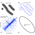
of grayscale gradients, which are typically particle edges, in the image. To illustrate, Figure 2A shows
a 50-by-50 pixel image of two gray stripes and a gray dot. At each pixel, there is a direction of
maximum grayscale brightness increase, and its length corresponds to the sharpness of the gradient.
These vectors are shown in Figure 2B; blank areas are where the brightness does not vary, and the
vectors have length zero. Most of the long brightness vectors point away from the centers of the
stripes, and a smaller number point at various other directions. In Figure 2C, all of the vectors from B
have been translated to the origin and rescaled. There is a clear concentration perpendicular to the
trends of the stripes, which defines the orientation of the long axis of the edge fabric ellipse (EFE;
Fig. 2D).
 Figure
2
Figure
2
(A) An image of gray stripes 50 pixels on a side. (B) Vectors showing magnitude and direction of the
brightness gradient at each pixel. (C) Vectors in B translated to the origin, showing strong grouping
perpendicular to dominant edges, along with scaled eigenvectors and ellipse defined by them. (D) Edge
fabric ellipse (EFE) derived by rotating ellipse in C 90°.
Axis lengths and orientations are computed using the eigenvectors and eigenvalues of the
variance-covariance matrix (Appendix 2). Because the vectors are oriented perpendicular to edges, and we
want the dominant edge direction, we simply rotate the ellipse 90° to produce the EFE (Fig. 2D). The
aspect ratio of the EFE, designated E, is a measure of the strength of the fabric defined by
edge alignment.
The EFE determined from grayscale gradients should be equivalent to the strain ellipse in the case of
deformation of a homogeneous material with passive markers. However, empirical tests show that for
images deformed digitally by pure shear,
E = Rk,
(1)
where R is the standard strain ratio (ratio of long and short axes of the strain ellipse), and
the exponent k typically lies in the range 1.2–1.5 for images of natural samples (e.g., granite
or sandstone). Because k > 1, the aspect ratio of the EFE, E, is less than that of
the strain ellipse, R. This is likely a consequence of image pixelization, and a full treatment
of this is beyond the scope of this paper.
Measuring Edge Fabric
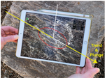
To determine EF, the user takes a photograph of a suitable rock face with the mobile device held parallel
to the face. The app then calculates the EFE. The tool gives a measure of the fabric’s magnitude by
reporting the axial ratio E of the ellipse and its orientation by giving the azimuth and trend
and plunge of its long axis (Fig. 3). Azimuth is the orientation of the long axis in the plane of the
device, and trend and plunge give the orientation of this line in space using the internal magnetometer,
gyroscope, and accelerometer of the mobile device to determine its attitude at the time an image is
captured. If the feature on the image is produced by, for example, the intersection of foliation with
the rock face, then the long axis of the EFE is an intersection lineation that lies in the foliation
plane.
 Figure
3
Figure
3
Using the edge fabric tool. The mobile device is held parallel to the plane being photographed. The app
calculates the edge fabric ellipse and reports its azimuth (long axis of the ellipse, relative to “up”
on the screen), its trend and plunge in space, and its axial ratio
E. Calculations take 5
seconds or less. The analysis can be captured as a screenshot, and the trend and plunge can be copied
for pasting into Stereonet Mobile (Allmendinger, 2019). StraboTools locks to landscape display.
Quantifying Strength of Fabric
Fabrics observed in the field can range from mylonites with simple shear strains in the thousands to
barely discernible foliations or pebble imbrications. Although the strength of mineral alignment,
shape-preferred orientation, and other features can be quantified in the lab, on the outcrop, one is
left with qualitative descriptions such as “strong fabric.”
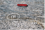
The EF tool gives a quantitative measure of fabric strength. In Figure 4, a shear zone comprises various
high-strain zones cutting weakly foliated granodiorite. By making EFEs in subareas, a gradation in
strength and orientation of fabric is clear. This can be done rapidly on the outcrop.
 Figure
4
Figure
4
Edge fabric ellipses of three subareas of this shear zone provide field-obtainable, objective measures
of fabric intensity and orientation. Shear zone cuts Jurassic granodiorite near Chickenfoot Lake, Sierra
Nevada, California, USA.
Making Fabric Measurement Portable and Fast
Perhaps the most commonly used text on quantitative strain analysis is Ramsay and Huber (1983) Sessions
5–8 (pages 73–149). They describe methods and give exercises appropriate to the sorts of rocks discussed
here, with the analyses commonly performed using the Fry (1979) center-to-center technique or the
Rf /Φ technique of Dunnet (1969). The former involves finding anticlustered markers
and graphing their center-to-center distances; the latter measuring the aspect ratios and elongation
directions of elliptical markers, and then finding a finite-strain ellipse that best explains them. Both
techniques are labor-intensive and subjective, even with image analysis and automation.
EFEs allow rapid analysis of deformed markers in the field or laboratory. Figures 5A–5D show three
artificial examples, and in each case, the EFE determined from StraboTools provides a close estimate of
the imposed strain. Figure 5C shows randomly oriented, randomly shaped ellipses, deformed by 10%
pure-shear stretching (strain ratio  )
along an azimuth of 065.The EFE (red) is almost coincident with the imposed strain ellipse (blue),
yielding an EFE aspect ratio E of 1.18 and an azimuth of 063. This is a classic subject for
Rf /Φ analysis, but it is difficult to see how one could infer the true deformation
(blue star in Fig. 5D) from the scatter of Rf /Φ points. The EFE solution (red star)
again aligns well with the true deformation.
)
along an azimuth of 065.The EFE (red) is almost coincident with the imposed strain ellipse (blue),
yielding an EFE aspect ratio E of 1.18 and an azimuth of 063. This is a classic subject for
Rf /Φ analysis, but it is difficult to see how one could infer the true deformation
(blue star in Fig. 5D) from the scatter of Rf /Φ points. The EFE solution (red star)
again aligns well with the true deformation.
 Figure
5
Figure
5
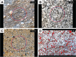
Examples of strain analysis using StraboTools. Red figures are edge fabric ellipses (EFEs) determined
with the app, and blue figures are the imposed deformation. (A) Artificial pattern from Waldron et al.
(2007), deformed along an undefined axis with strain ratio
R = 1.3; the edge fabric tool gives
E = 1.21 with an elongation azimuth of 133°. Correcting using Equation 1 with
k = 1.3
gives , very close to imposed strain. (B) Cross-polarized thin section view of an isotropic aplite dike
deformed by 20% shortening in the vertical direction and 25% stretching in the horizontal (
R =
1.56), with EFE (, which corrects with Equation 1–1.56). (C) Ellipses with random axial ratios and
orientations that were stretched 10% along an azimuth of 065. Agreement between the imposed strain
(blue) and computed EFE (red) strain is excellent. (D)
Rf /Φ plot of data from C,
with the imposed deformation and EFE solutions indicated by stars. It is hard to see how one could infer
the imposed deformation (blue star) from the scatter of points, but the EFE solution matches it well.
(E) Thin section view of deformed quartzite from Ramsay and Huber (1983, p. 118). (F) Their Fry plot
derived from it, with EFE. The EFE agrees well with the elliptical void.
Figure 5E is a thin-section view of deformed quartzite from Ramsay and Huber (1983, their
figure 7.16, p. 118). Their Fry plot is given in Figure 5F along with the EFE. In such a plot, the shape
of the hole in the center is an estimate of the strain ellipse. Ramsay and Huber (1983, p. 124) noted,
“It is not an easy matter to identify with confidence the dimensions of the elliptical form of the point
data,” highlighting the subjectivity involved in determining R. The EFE provides a good fit to
the Fry plot and is an objective measure of the fabric.
EFEs have utility in other fields as well. At the micro scale they allow measurement of orientation and
strength of microlite alignment, vesicle elongation, compaction fabric, and other textural features in
thin section. At the macro scale they offer a way to measure and quantify the orientation and frequency
of joints, dikes, and other features on aerial photographs. Because of its speed and ease of use,
StraboTools makes taking many measurements a practical and efficient reconnaissance exercise.
Caveats
It is important to note that the EFE is simply a measure of the preferred orientation of grayscale
gradients in the image. If we take a homogeneous image to start, whether it be a rock or artificial
random pattern of circles, E correlates with the distortion we apply to the image, which
approximates the finite strain.
Sedimentary compositional or textural banding typically produces EFEs with large Es, but these
are not a result of deformation. In thin section, plagioclase twinning, perthitic texture, and other
phenomena will generate edge alignments that are unrelated to deformation. In these cases, however, the
EFE is still a quantitative measure of edge alignment and fabric in the image. Conversely, many fabric
patterns that are obvious to the eye will be invisible to EFE analysis. For example, alternating layers
of black and white circles will produce an isotropic EFE, even though layering is quite apparent.
E values are not necessarily equal to the finite strain. As reviewed in Ramsay and Huber (1983),
determining finite strain means understanding all of the possible deformation mechanisms (e.g., creep,
grain-boundary sliding, etc.). StraboTools does not give this information, but E correlates
with strain, and the EFE aligns well with fabric, even fabrics that are too subtle to see (Fig. 1). For
an igneous rock, the EFE may capture a subtle grain shape fabric or crystal alignment not evident in the
field.
There are several cautions about using EFEs. First, they are highly sensitive to shadows and cracks or
fractures. In tests on glacially polished outcrops, a low sun angle can produce an elongate EFE whose
axis is perpendicular to the sun azimuth even when visible shadows are not apparent. It is good practice
to work with evenly shadowed surfaces. Second, although one can snap photos of images from computer
screens, many artifacts, such as moiré patterns and the rectangular nature of pixels, can affect the
results. High-resolution original images should be used whenever possible.
Color Index
Color index (CI), the volume percent of dark minerals visible in an outcrop of plutonic rock, is commonly
estimated in the field. In granitic rocks, dark minerals such as biotite, hornblende, clinopyroxene,
Fe-Ti oxides, and titanite are commonly easy to observe, but estimating their percentage by eye,
especially when the percentage is small, is a notoriously difficult endeavor even for experienced
observers. Comparison charts (Folk, 1951; Compton, 1985) are helpful, but it is still difficult to
estimate CI accurately or precisely by eye, with visual psychology playing a prominent role in
introducing biases (Allen, 1956; Dennison and Shea, 1966).
Accurate measurement of CI in the field could allow the delineation of zoning patterns that previously
required laboratory or thin-section analysis. For example, the Half Dome and Cathedral Peak plutons in
Yosemite National Park form a gradationally nested pair with a consistent inward decrease in CI that
accompanies significant parallel changes in bulk composition (Bateman et al., 1988). The Cathedral Peak
Granodiorite ranges from CI ~10 and SiO2 ~68 wt% at its outer contact to CI ~4 and
SiO2 ~72 wt% at its inner. The gradual factor-of-two variation in CI is well within the
typical error range of visual CI estimates (see Fig. 1D) and would be difficult to pick up by visual
means alone.
The CI tool (Fig. 6) provides a rapid, precise, and accurate tool for estimating CI. In practical use on
suitable rock faces, CI is typically reproducible within 1 or 2 absolute percent (e.g., 15 ± 2). The
values determined by the CI tool match those determined by point counting within the same range.
 Figure
6
Figure
6
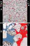
The color index (CI) tool in use. The user takes a photograph of a clean, shadow-free rock face and then
uses the slider (lower left) to highlight the desired pixels in red or blue. (A) Determination of CI in
a leucocratic granodiorite. The CI is displayed at upper right. A portion of the highlighted pixels has
been erased to show the unhighlighted image below. (B) Using the CI tool for quick estimation of the
percentage of porosity, as represented by blue epoxy, in a sandstone. The left half of the image is the
original photomicrograph; on the right half the slider has been adjusted to highlight the epoxy. Dark
inclusions represent ~3% of the image (as determined with the slider); thus, the porosity is 40%.
Photomicrograph by Michael C. Rygel.
Field Geology in 2020 and Beyond
Using StraboTools can significantly enhance the practice of field geology by providing objective ways to
collect data types that are impractical or impossible to collect in the field, subject to poor
precision, or arduous and time-consuming to do later in the lab. StraboTools lets the field geologist
examine rock fabrics in situ or back in the lab with thin sections or cut slabs. Because the app
requires the user to capture an image and work on that same picture, it can be used to thoroughly
document the data collected and can be reproduced or tested on the same source by other scientists. The
tools also record the location and orientation of the image, so it becomes more practical to reproduce
the actual field observations at a later date.
In his Presidential Address to the Geological Society of America, “New Technology; New Geological
Challenges,” B.C. Burchfiel (2003 [published in 2004]) made a compelling case that the geological
community must embrace new modes of data collecting. At that time, precise GPS measurements were
revolutionizing active tectonics and opening entirely new avenues of research. Developing and adopting
new mobile technology can advance our ability to perform basic field geology at the individual
investigator level. Images and interpretations can be easily shared, discussed, and interpreted by
scientists and the interested public. Citizen scientists could have a role in collecting and evaluating
geologic data in ways similar to that done for plants and animals with iNaturalist (https://www.inaturalist.org), with over 275,000 species identified,
and eBird (https://ebird.org),
with more than 100,000,000 bird sightings each year.
Sharing Data
We envision that StraboTools will lead to more sharing of data and make fieldwork more transparent,
reproducible, and searchable. StraboTools was developed as a spinoff of the StraboSpot project, which
allows field geologists to collect, store, and share geologic data more easily. StraboSpot is currently
focused on collecting general field data for structural geology, petrology, sedimentary geology, and
volcanology (Walker et al., 2019). Although not yet a direct part of StraboSpot, StraboTools data and
images can be entered into StraboSpot and StereonetMobile (Allmendinger et al., 2017).
Summary
We have developed a mobile app that allows field geologists to make quantitative measurements of features
such as foliation orientation and intensity, mineral alignment, and mineral proportions rapidly,
precisely, and reproducibly. The app can pick up subtle fabrics (e.g., weak foliation, flow alignment,
or pebble imbrication) that can be difficult to see. It allows objective measurement of features that
were heretofore subjectively evaluated or just not seen, and can be used to quantify fabrics in
photomicrographs and aerial photographs. It rapidly and objectively performs fabric analyses that were
formerly time-consuming, subjective, and of low precision.
Acknowledgments
Jason Ash is a crucial partner in this effort, doing the hard work of turning Matlab code into a stable
app. We thank all the participants at various StraboSpot workshops and field trips for their input into
how to improve the app. We thank an anonymous reviewer and editor Peter Copeland for reviews that
greatly improved the presentation. John Bartley and Kevin Stewart were valuable sounding boards during
development, and they and Andreas Möller provided constructive reviews of the manuscript. This work was
supported in part by National Science Foundation grants EAR 1639724 to AFG and EAR 1347331, ICER
1639734, and ICER 1639738 to JDW, and by the Mary Lily Kenan Flagler Bingham Professorship at the
University of North Carolina.
Appendix 1
 Puzzle Answers
Screenshots of answers to the puzzles in Figure 1. Blue circles are for reference. (A) Foliation in
deformed granite (Inyo Range, California, USA) has an edge fabric ellipse (EFE) aspect ratio
(
E) of 1.28 at an azimuth of 070 in the photo. (B) This image of granodiorite (Yosemite
National Park, California, USA) was deformed by pure-shear stretch of 10% along a bearing of 030
(
R = 1.22); EFE gives
E = 1.11 along 030. (C) Shadowed vertical face cut into alluvial
deposits (Death Valley National Park, California, USA), downstream to right, yields an EFE long axis
rotated 20° counterclockwise from horizontal. The camera was held with a horizontal horizon, and
layering is essentially horizontal, but EFEs in this and several other photos of the same face are
consistently aligned with their long axes rotated 20° to 30° counterclockwise from horizontal. We
attribute this to pebble imbrication and suggest that EFEs may aid the detection of these subtle
fabrics. (D) Color index determination on this granodiorite (Peninsular Ranges, California, USA) yields
9% dark minerals. EFE (not shown) detects the rather obvious steep fabric defined by alignment of the
dark minerals. See the original photos in the Supplemental Material.
1
Appendix 2
Calculation of Edge Fabric
At each pixel in an image, there is a direction of maximum grayscale brightness increase. We compute this
vector at each point by convolving the grayscale image with a 3-by-3 Sobel kernel (Sobel and Feldman,
1968) to get the horizontal brightness gradient at each pixel, and with the transpose of the kernel to
get the vertical gradient. Vectors defined by these two components are shown in Figure 2B.
The StraboTools app downsamples the image to 1000 pixels on the long edge. Hence, a typical image has
106 pixels, at each of which there is a horizontal and vertical component of gradient. We
form a 2-by-2 variance-covariance matrix from this 106-by-2 gradient matrix and calculate its
eigenvectors and eigenvalues. These eigenvectors, scaled by the corresponding eigenvalues’ square roots,
are plotted in Figure 2C along with the ellipse that they define. As the vectors point perpendicular to
edges, and we want the dominant edge direction, we rotate the ellipse 90° to produce the EFE (Fig. 2D).
The aspect ratio of the EFE is given by the square root of the ratio of the eigenvalues of the
variance-covariance matrix. The eigenvalues are the variances of the data projected onto the
corresponding eigenvectors; the longer eigenvector is the direction that maximizes this projected
variance (Dunteman, 1989, p. 29), and we take square roots to convert to the actual data spread
(standard deviation). The aspect ratio is thus the ratio of the data spread in the direction of the
longer eigenvector to that in the direction of the shorter eigenvector (Spruyt, 2014).
References Cited
- Ailleres, L., and Champenois, M., 1994, Refinements to the Fry method (1979) using image processing:
Journal of Structural Geology, v. 16, p. 1327–1330, https://doi.org/10.1016/0191-8141(94)90073-6.
- Allen, J.E., 1956, Estimation of percentages in thin sections—Considerations in visual psychology:
Journal of Sedimentary Petrology, v. 26, p. 160–161,
https://doi.org/10.1306/74D704F7-2B21-11D7-8648000102C1865D.
- Allmendinger, R., 2019, Stereonet Mobile: version 3.4.1 [mobile application software]: Retrieved
from https://apps.apple.com/us/app/stereonet-mobile/id1194772610.
- Allmendinger, R.W., Siron, C.R., and Scott, C.P., 2017, Structural data collection with mobile
devices: Accuracy, redundancy, and best practices: Journal of Structural Geology, v. 102, p. 98–112,
https://doi.org/10.1016/j.jsg.2017.07.011.
- Aydin, A., Ferré, E.C., and Aslan, Z., 2007, The magnetic susceptibility of granitic rocks as a
proxy for geochemical composition: Example from the Saruhan granitoids, NE Turkey: Tectonophysics,
v. 441, p. 85–95, https://doi.org/10.1016/j.tecto.2007.04.009.
- Bateman, P.C., Chappell, B.W., Kistler, R.W., Peck, D.L., and Busacca, A.J., 1988, Tuolumne Meadows
Quadrangle, California; analytic data: U.S. Geological Survey Bulletin, v. 1819, p. 43.
- Burchfiel, B.C., 2004, New technology; new geological challenges: GSA Today, v. 14, p. 4–10,
https://doi.org/10.1130/1052-5173(2004)014<0004.
- Coleman, D.S., Bartley, J.M., Glazner, A.F., and Pardue, M.J., 2012, Is chemical zonation in
plutonic rocks driven by changes in source magma composition or shallow-crustal differentiation?:
Geosphere, v. 8, https://doi.org/10.1130/GES00798.1.
- Compton, R.R., 1985, Geology in the Field: New York, Wiley, 398 p.
- Dennison, J.M., and Shea, J.H., 1966, Reliability of visual estimates of grain abundance: Journal of
Sedimentary Petrology, v. 36, p. 81–89.
- Dühnforth, M., Anderson, R.S., Ward, D., and Stock, G.M., 2010, Bedrock fracture control of glacial
erosion processes and rates: Geology, v. 38, p. 423–426, https://doi.org/10.1130/G30576.1.
- Dunnet, D., 1969, A technique of finite strain analysis using elliptical particles: Tectonophysics,
v. 7, p. 117–136, https://doi.org/10.1016/0040-1951(69)90002-X.
- Dunteman, G.H., 1989, Principal components analysis (Sage University paper series on quantitative
applications in the social sciences, no. 69): London, SAGE, 96 p.
- Folk, R.L., 1951, A comparison chart for visual percentage estimation: Journal of Sedimentary
Petrology, v. 21, p. 32–33.
- Fry, N., 1979, Random point distributions and strain measurement in rocks: Tectonophysics, v. 60, p.
89–105, https://doi.org/10.1016/0040-1951(79)90135-5.
- Launeau, P., Bouchez, J.L., and Benn, K., 1990, Shape preferred orientation of object populations:
Automatic analysis of digitized images: Tectonophysics, v. 180, p. 201–211,
https://doi.org/10.1016/0040-1951(90)90308-U.
- Parkinson, D.N., 1996, Gamma-ray spectrometry as a tool for stratigraphical interpretation: Examples
from the western European Lower Jurassic, in Hesselbo, S.P., and Parkinson, D.N., eds.,
Sequence Stratigraphy in British Geology: Geological Society (London) Special Publication 103, p.
231–255, https://doi.org/10.1144/GSL.SP.1996.103.01.13.
- Ramsay, J.G., and Huber, M.I., 1983, The Techniques of Modern Structural Geology, Volume 1: Strain
Analysis: London, Academic Press, 307 p.
- Sobel, I., and Feldman, G., 1968, A 3 × 3 isotropic gradient operator for image processing: A talk
at the Stanford Artificial Project in 1968, p. 271–272.
- Spruyt, V., 2014, A geometric interpretation of the covariance matrix:
https://www.visiondummy.com/2014/04/geometric-interpretation-covariance-matrix/ (accessed 15 Feb.
2020).
- Vinta, B.S.S.R., and Srivastava, D.C., 2012, Rapid extraction of central vacancy by image-analysis
of Fry plots: Journal of Structural Geology, v. 40, p. 44–53,
https://doi.org/10.1016/j.jsg.2012.04.004.
- Walker, J.D., Tikoff, B., Newman, J., Clark, R., Ash, J.M., Good, J., Bunse, E.G., Möller, A., Kahn,
M., Williams, R., Michels, Z., Andrew, J.E., and Rufledt, C., 2019, StraboSpot data system for
structural geology: Geosphere, v. 15, https://doi.org/10.1130/GES02039.1.
- Waldron, J.W.F., and Wallace, K.D., 2007, Objective fitting of ellipses in the centre-to-centre
(Fry) method of strain analysis: Journal of Structural Geology, v. 29, p. 1430–1444,
https://doi.org/10.1016/j.jsg.2007.06.005.